PWA and Boxcar Averager
Note
This tutorial is applicable to UHF Instruments with the UHF-BOX Boxcar Averager option installed.
Goals and Requirements
This tutorial explains how to set up a periodic waveform analyzer (PWA) and a boxcar averager for measuring periodic signals with low duty cycles. The advantages of using the PWA and the boxcar averager over a digital scope or a lock-in amplification technique will be explained and demonstrated as follows.
The duty cycle and the signal energy that is available in the fundamental frequency scale almost linearly. For example, a rectangular signal pulse with 50% duty cycle has only 1/3 of the signal amplitude in the fundamental frequency. And if the duty cycle is further halved, then the signal in the fundamental is also halved. Hence, lock-in amplification, which normally references to the fundamental frequency, may not always be the best way to recover a signal if the pulse waveform has a duty cycle smaller than 50%. In this case, boxcar averaging may be the more efficient measurement method. If the signal spreads out over many harmonic components without any prominent peak, a boxcar detection scheme might be the wiser choice to achieve the best possible signal-to-noise ratio.
To perform the measurements in this tutorial, one will require a 3rd-party programmable arbitrary waveform/function generator for narrow pulse generation.
Preparation
Connect the cables as described below. Make sure that the UHF unit is powered on and connected by USB to your host computer or by Ethernet to your local area network (LAN) where the host computer resides. After starting LabOne the default web browser opens with the LabOne graphical user interface.

The tutorial can be started with the default instrument configuration (e.g. after a power cycle) and the default user interface settings (e.g. as is after pressing F5 in the browser).
Low Duty Cycle Signal Measurement
There are a couple of ways to measure a low duty cycle signal with the UHF instrument. The obvious method is to use the Scope function inside the LabOne interface to observe the sampled signal in the time domain. The other method is to use the PWA and the boxcar averager. Both methods will be shown. The first task is to generate a test signal.
Narrow Pulse Signal Generation
Using the external arbitrary waveform generator, generate a pulse with the following specifications.
| Pulse Specification | Section |
|---|---|
| Pulse Type | Square |
| Amplitude | 100 mVpp |
| Frequency | 9.7 MHz |
| Duty Cycle | < 16% |
Note
For this exercise, an Agilent 33500B Truefrom waveform generator is used. The minimum duty cycle for a 9.7 MHz signal on this instrument is about 16%.
The LabOne Scope can be used to observe the generated pulse waveform. Connect the output of the AWG directly to Signal Input 1 of the UHF instrument. The Scope settings in LabOne are given in the table below. Also, the AWG should also be able to provide a TTL synchronization signal to be connected to the Ref / Trigger input. This trigger signal will be used later on for the PWA.
| Tab | Sub-tab | Section | # | Label | Setting / Value / State |
|---|---|---|---|---|---|
| Lock-in | All | Signal Inputs | 1 | AC | OFF |
| Lock-in | All | Signal Inputs | 1 | 50 Ω | ON |
| Lock-in | All | Signal Inputs | 1 | Range | 200.0 m |
| Scope | Control | Vertical | Channel 1 | Signal Input 1/ON | |
| Scope | Trig | Trigger | Signal | Signal Input 1/ON | |
| Scope | Trig | Trigger | Enable | ON | |
| Scope | Trig | Trigger | Level | 30.0 m | |
| Scope | Trig | Trigger | Hysteresis | 10.0 m | |
| Scope | Run/Stop | ON |
One should now be able to observe Signal Input 1 similar to the following waveform in the Scope window. The Scope is set to self trigger on the pulse edges. Use the horizontal zoom to focus on a single period. This can be done by rolling the mouse wheel forward to zoom in the horizontal axis. To zoom in on the vertical axis, press down the Shift key and roll the mouse wheel. One can also recenter the waveform by pressing on the left mouse button and dragging the Scope plot area.
One can observe that the shape of the supposedly square pulse does not have sharp edges as one would expect. This is due to the effect of the 600 MHz low pass filter at the input of the UHF instrument. In fact, the signal input bandwidth of 600 MHz corresponds to about 1.5 ns rise time (20% - 80%). Here, the sampled pulse width shown in the Scope is measured to be about 29 ns or 30% duty cycle. The smeared out waveform has a duty cycle bigger than the 16% that was originally set.
![]()

Low Duty Cycle Analysis with Period Waveform Analyzer
To analyze the pulse waveform using the PWA, the UHF instrument first has to lock to the trigger signal of the pulses. This is done using the Ext Ref mode. The trigger signal is fed to the Ref / Trigger connector on the front panel which can be an analog signal or a TTL signal. The trigger level can be adjusted in the DIO tab as shown in Using Ref / Trigger Input and Output for Referencing. To lock to the trigger signal, use the Lock-in tab settings in the table below. The goal is to lock the internal oscillator 1 to the external trigger from the AWG. The frequency of oscillator 1 in the Lock-in tab should now display 9.7 MHz, with the green light indicating a lock condition.
| Tab | Sub-tab | Section | # | Label | Setting / Value / State |
|---|---|---|---|---|---|
| Lock-in | All | Reference | 4 | Mode | ExtRef |
| Lock-in | All | Demodulators Input | 4 | Signal | Trigger 1 |
To activate the PWA function, place one instance of the Boxcar tab in the LabOne web interface. To display the 9.7 MHz pulse over a single period, the following parameters need to be set.
| Tab | Sub-tab | Section | # | Label | Setting / Value / State |
|---|---|---|---|---|---|
| Boxcar | PWA | Signal Input | 1 | Input Signal | Sig In 1/ON |
| Boxcar | PWA | 1 | Run/Stop | ON |
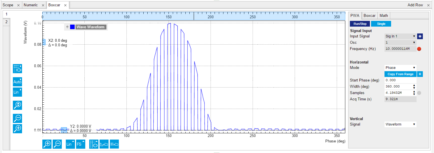
Immediately, one can see in the PWA a very stable and smooth peak in one pulse period. The horizontal axis is shown in phase over 360 degrees to represent one period of the pulse waveform. The position of the peak also indicates the precise phase delay with respect to the trigger signal. In this phase representation, the PWA divides the full 360 degrees into 1024 bins. The phase resolution is therefore about 0.35 deg; for a signal of 9.7 MHz this corresponds to a time resolution of about 100 ps.
![]()

If this resolution is not sufficient, one can use the Zoom mode. By reducing the Width (deg), one can get more details of the characteristics of the pulse. The redefined phase range will then again be divided into 1024 bins. To acquire the same number of samples for a smaller Width requires a longer acquisition time.
Note
The Zoom mode references the input signal to a higher harmonic of the reference frequency which allows zooming into the region of interest, and hence increasing the temporal resolution down to millidegrees. This gives a precise analysis for pulsed signals with low duty cycles or any other periodically repeating transient. Of course the real resolution is still limited by the signal input bandwidth, as in the case of the Scope.
![]()

Beside the phase domain display, one can also choose the horizontal display axis in the unit of time or frequency. The harmonics of the pulse waveform can also be analyzed by setting Mode to Harmonics. These options are all part of the multi-channel, multi-domain PWA for peak analysis.
The frequency of 9.7 MHz is not chosen accidentally. In general, one should avoid choosing a modulation frequency that shares the same divisor as the maximum UHF-BOX repetition rate of 450 MHz i.e. the two numbers should not be commensurable. For example, 10 MHz and 450 MHz are commensurable since they can be both divided by 10. This commensurability issue arises from the internal digital signal processing which may cause certain bins to get filled constantly but not others. Such an example is shown in the figure below. A red warning indicator will be switched on when a potential commensurability problem is detected.
Low Duty Cycle Analysis with Scope
The digitized waveform in the Scope can be jittery and noisy. One must remember that the pulse is sampled at 1.8 GSa/s which corresponds to a minimum resolution of 555 ps. This resolution implies that in the zero-crossing triggering, the triggered point on the waveform will not be the same for every pulse. This is indeed one major source of jitter observed.
The Scope comes with averaging and the persistence function which can in theory help to minimize jitter and noise. To use the averaging mode, one simply has to set Avg Filter field under the Scope Control tab to Exp Moving Avg. Then one can choose the number of Averages desired. Below is the averaged pulse waveform at 10 points. Compared to the previous non-averaged waveform, it can be seen that now the spikes are smoothed out.
![]()

In order to observe the extent of jitter and noise, one can use the Persistence mode. Persistence can be enabled in the Advanced sub-tab. Enabling persistence causes each triggered waveform to be superimposed on top of the previous ones. The result of the persistence is shown in the graph below where the superimposed traces are in red. Under this condition, the Scope method can be said to be not an ideal tool to analyze a narrow peak, especially when the peak width would be below a nanosecond.
Note
Persistence cannot be used simultaneously with averaging.
![]()

Comparison shows that the PWA tool is a more precise and elegant way to analyze this type of narrow pulse waveform.
Boxcar Integration
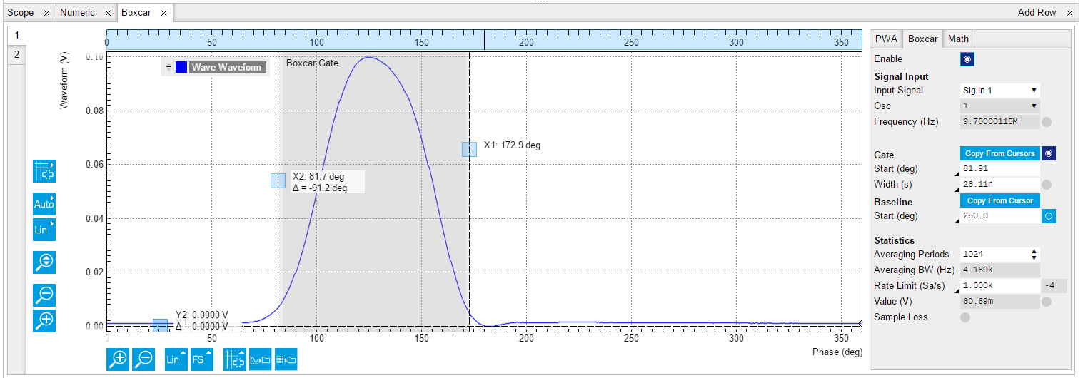
The boxcar averager can be configured in the Boxcar sub-tab. The boxcar averager integrates and normalizes a section of the signal and generates an output signal in units of volt. The integrated gate can be set either manually in the Start Phase (deg) and Width (deg) fields, or by positioning to vertical cursors and then clicking Copy From Cursor. The integrated value is updated in the Value (V) field. An example boxcar setting is shown below. Choosing a boxcar window roughly equal to the pulse width usually yields the best signal-to-noise ratio.
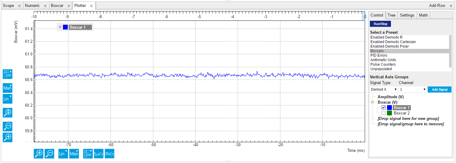
The result of the integration can also be shown graphically using the Plotter tool as shown below.
![]()
Baseline Suppression
It may happen that a low-frequency noise signal is visible on the boxcar output signal. This noise can come from the power supply, emf noise coupled through the external wirings or even from the experiment itself. In this case, the baseline suppression function can be applied to remove the undesired noise found in the Boxcar integration. To show the benefits of the baseline suppression, the following connections can be made to simulate an undesired period noise injection. In this example, the UHF Signal Output 1 is used to generated a 100 Hz sine wave superimposed on top of the AWG waveform through a T-connector.

| Tab | Sub-tab | Section | # | Label | Setting / Value / State |
|---|---|---|---|---|---|
| Lock-in | All | Oscillators | 2 | Frequency | 100 Hz |
| Lock-in | All | Output Amplitudes | 2 | Amp 1(Vpk) | 0.3 |
| Lock-in | All | Signal Outputs | Output 1 | ON |
When this is done, the Plotter tool will display an integrated value with the 100 Hz sine component instead of the flat line shown previously.
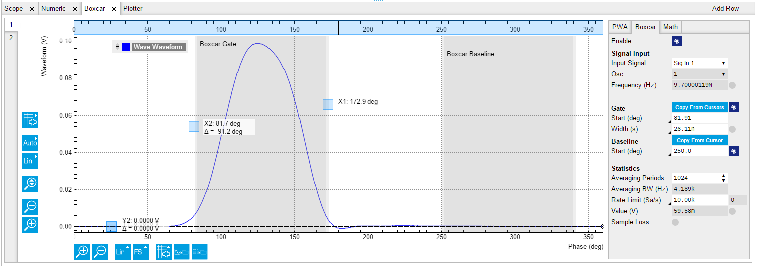
This undesired sine variation can be eliminated using the Baseline settings in the Boxcar sub-tab. The baseline subtraction window has the same width as the Boxcar integration window. When enabling baseline subtraction, the window position is shown in the PWA waveform just like the integration window. The baseline window should be chosen outside of the pulse in order to subtract only the superimposed sine, and not the signal.
![]()
Once baseline subtraction is enabled and the baseline window is defined suitably, the Plotter will show that the sine component has disappeared. The trace that is left is equal to the original Boxcar averager value.
![]()

![]()

With enabled Baseline suppression, the operating frequency of the Boxcar Averager is limited to 450 MHz. There is, however, a trick to use it at higher frequencies by combining both Boxcar Averager units. The idea is to measure at exactly half the frequency. By setting the Harmonic of the demodulator used to lock to an external reference to 2, it will generate a sub-harmonic of the external reference on it’s associated oscillator (e.g. oscillator 1). Both boxcar averagers and PWAs are then configured to measure with this oscillator reference. The two PWA will each show two periods (i.e. peaks) of the signal. The first Boxcar Averager gate should be centered around the first peak, the second Boxcar Averager gate around the second peak. The baseline suppression gates should be individually selected. The two Boxcar Averager output signals can then be added up in the Arithmetic Unit (AU) tab. This setup corresponds then to a full Boxcar Averager operating above 450 MHz.