Arbitrary Waveform Generator¶

Note

This tutorial is applicable to UHFLI Instruments with the UHF-AWG Arbitrary Waveform Generator option installed and to UHFAWG Instruments. Where indicated, additional options such as UHF-DIG, UHF-BOX, UHF-CNT, UHF-MF, or UHF-LIA are required.

Goals and Requirements¶

The goal of this tutorial is to demonstrate the basic use of the AWG. We demonstrate waveform generation and playback, triggering and synchronization, carrier modulation, and sequence branching. We conclude with a list of tips for operating the AWG. The measurements in this tutorial can be performed using simple loop back connections.

Preparation¶

Connect the cables as illustrated below. Make sure that the UHF unit is powered on and connected by USB to your host computer or by Ethernet to your local area network (LAN) where the host computer resides. After starting LabOne, the default web browser opens with the LabOne graphical user interface.

Figure 1: UHF connections for the arbitrary waveform generator tutorial

The tutorial can be started with the default instrument configuration (e.g. after a power cycle) and the default user interface settings (e.g. as is after pressing F5 in the browser).

Waveform Generation and Playback¶

In this tutorial we generate arbitrary signals with the AWG and visualize them with the Scope. In a first step we enable the Signal Outputs, but disable all sinusoidal signals generated by the lock-in unit by default. We also configure the Scope signal input and triggering and arm it by clicking on in the Scope. The following table summarizes the necessary settings.

Table 1: Settings: enable the output and configure the Scope
Tab	Sub-tab	Section	#	Label	Setting / Value / State
In/Out		Signal Outputs	1	Enable	ON
In/Out		Signal Outputs	2	Enable	ON
Lock-in	All	Output Amplitudes	1-8	Amp 1 Enable	OFF
Lock-in	All	Output Amplitudes	1-8	Amp 2 Enable	OFF
Scope	Control	Vertical		Channel 1	Signal Input 1
Scope	Trigger	Trigger		Enable	ON
Scope	Trigger	Trigger		Signal	Signal Input 1
Scope	Trigger	Trigger		Level	0.1 V
Scope	Control			Run/Stop	ON

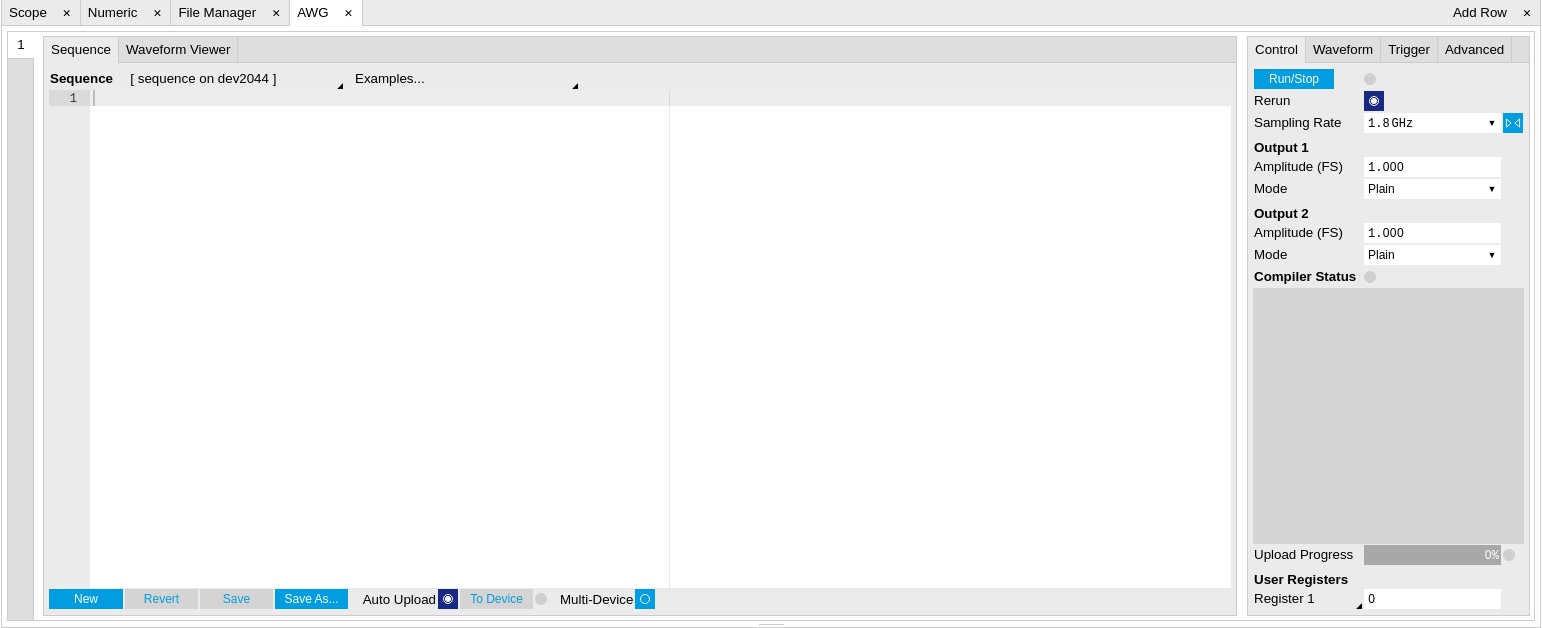
In the AWG tab, we configure both channels to output signals at the full scale (FS) in plain output mode as summarized in the following table.

Table 2: Settings: configure the AWG output
Tab	Sub-tab	Section	Label	Setting / Value / State
AWG	Control		Rate (Sa/s)	1.8 GHz
AWG	Control		Rerun	OFF
AWG	Control	Output 1	Amplitude (FS)	1.0
AWG	Control	Output 1	Mode	Plain
AWG	Control	Output 2	Amplitude (FS)	1.0
AWG	Control	Output 2	Mode	Plain

Operating the AWG means first of all to specify a sequence program. This can be done interactively by typing the program in the Sequence Editor window. Let’s start by typing the following code into the Sequence Editor.

wave w_gauss = 1.0*gauss(8000, 4000, 1000);
playWave(1, w_gauss);

In the first line of the program, we generate a waveform with a Gaussian shape with a length of 8000 samples and store the waveform under the name w_gauss. The peak center position 4000 and the standard deviation 1000 are both defined in units of samples. You can convert them into time by dividing by the chosen Rate (1.8 GSa/s by default). The waveform generated by the gauss function has a peak amplitude of 1. This amplitude is dimensionless and the physical signal amplitude is given by this number multiplied with the signal output range (e.g. 1.5 V). We put a scaling factor of 1.0 in place which can be replaced by any other value below 1. The code line is terminated by a semicolon according to C conventions. In the second line, the generated waveform w_gauss is played on AWG Output 1.

Note

For this tutorial, we will keep the description of the Sequencer commands short. You can find the full specification of the LabOne Sequencer language in LabOne Sequence Programming

Note

The AWG has a waveform granularity of 16 samples. It’s recommended to use waveform lengths that are multiples of 16, e.g. 8000 like in this example, to avoid having ill-defined samples between successively played waveforms. Other waveform lengths are allowed, though.

If we now click on , the program gets compiled. This means the program is translated into instructions for the LabOne Sequencer on the UHF instrument, see AWG Tab. If no error occurs (due to wrong program syntax, for example), the Status LED lights up green, and the resulting program as well as the waveform data is written to the instrument memory. If an error or warning occurs, messages in the Status field will help in debugging the program. If we now have a look at the Waveform sub-tab, we see that our Gaussian waveform appeared in the list. The Memory Usage field at the bottom of the Waveform sub-tab shows what fraction of the instrument memory is filled by the waveform data. The Waveform viewer sub-tab allows you to graphically display the currently marked waveform in the list.

By clicking on with Rerun disabled, we have the AWG execute our program once. Since we have armed the Scope previously with a suitable trigger level, it has captured our Gaussian pulse with a FWHM of about 1.33 μs as shown in Figure 3.

Figure 3: Gaussian pulse as generated by the AWG and captured by the LabOne Scope

The LabOne Sequencer language contains various control structures. The basic functionality is to play back a waveform several times. In the following example, all the code within the curly brackets '{...}' is repeated 5 times. Upon clicking and you should observe 5 short Gaussian pulses in a new scope shot, see Figure 4 .

wave w_gauss = 1.0 * gauss(640, 320, 50);

repeat (5) {
  playWave(1, w_gauss);
}

Figure 4: Burst of Gaussian pulses generated by the AWG and captured by the LabOne Scope

In order to generate more complex waveforms, the LabOne Sequencer programming language offers a rich toolset for waveform editing. On the basis of a selection of standard waveform generation functions, waveforms can be added, multiplied, scaled, concatenated, and truncated. It’s also possible to use compile-time evaluated loops to generate pulse series with systematic parameter variations – see LabOne Sequence Programming for more precise information. In the following code example, we make use of these tools to generate a pulse with a smooth rising edge, a flat plateau, and a smooth falling edge. We use the cut function to cut a waveform at defined sample indices, the rect function to generate a waveform with constant level 1.0 and length 320, and the join function to concatenate three (or arbitrarily many) waveforms.

wave w_gauss = gauss(640, 320, 50);
wave w_rise = cut(w_gauss, 0, 319);
wave w_fall = cut(w_gauss, 320, 639);
wave w_flat = rect(320, 1.0);

wave w_pulse = join(w_rise, w_flat, w_fall);

while (true) {
  playWave(1, w_pulse);
}

Note that we replaced the finite repetition by an infinite repetition by using a while loop. Loops can be nested in order to generate complex playback routines. The Rerun button in the Control sub-tab will simply cause the entire AWG program to be restarted automatically. This is a simple alternative for creating loops, however, unlike the while loop the Rerun method does not allow back-to-back waveform playback and comes with a certain timing jitter. The output generated by the program above is shown in Figure 5.

Figure 5: Infinite pulse series generated by the AWG and captured by the LabOne Scope

One pitfall when using loops has to do with the nature of the playWave and related commands. This command initiates the waveform playback, but during the playback the sequencer will start to execute the next command on his list. This is useful as it allows you to execute commands during playback. In a loop, it means the sequencer can jump back to the beginning of the loop while the waveform is still being played. You can easily change this behavior by adding waitWave as the last command in the loop.

As programs get longer, it becomes useful to store and recall them. Clicking on allows you to store the present program under a newly chosen file name. Clicking on then saves your program to the file name displayed at the top of the editor. As you begin to work on sequence programs more regularly, it’s worth expanding your repertoire by some of the editor keyboard shortcuts listed in Sequence Editor Keyboard Shortcuts.

It’s also possible to iterate over the samples of a waveform array and calculate each one of them in a loop over a compile-time variable cvar. This often allows to go beyond the possibilities of using the predefined waveform generation function, particularly when using nested formulas of elementary functions like in the following example. The waveform array needs to be pre-allocated e.g. using the instruction zeros.

const N = 1024;
const width = 100;
const position = N/2;
const f_start = 0.1;
const f_stop = 0.2;
cvar i;
wave w_array = zeros(N);
for (i = 0; i < N; i++) {
  w_array[i] = sin(10/(cosh((i-position)/width)));
}

playWave(w_array);

Should you require more customization than what is offered by the LabOne AWG Sequencer language, you can import any waveform from a comma-separated value (CSV) file. The CSV file should contain floating-point values in the range from –1.0 to +1.0 and contain one or several columns, corresponding to the number of channels. As an example, the following could be the contents of a file wave_file.csv specifying a dual-channel wave with a length of 16 samples:

  -1.0   0.0
  -0.8   0.0
  -0.7   0.1
  -0.5   0.2
  -0.2   0.3
  -0.1   0.2
 0.1   0.0
 0.2    -0.1
 0.7    -0.3
 1.0    -0.2
 0.9    -0.3
 0.8    -0.2
 0.4    -0.1
 0.0    -0.1
  -0.5    -0.1
  -0.8   0.0

Store the file in the location of C:\Users\<user name>\Documents\Zurich Instruments\LabOne\WebServer\awg\waves\wave_file.csv under Windows or ~/Zurich Instruments/LabOne/WebServer/awg/waves/wave_file.csv under Linux. In the sequence program you can then play back the wave by referring to the file name without extension:

playWave("wave_file");

If you prefer, you can also store it in a wave data type first and give it a new name:

wave w = "wave_file";
playWave(w);

The external wave file can have arbitrary content, but consider that the final signal will pass through the 600 MHz low-pass filter of the instrument. This means that signal components exceeding the filter bandwidth are not reproduced exactly as suggested for example by looking at a plot of the waveform data. In particular, this concerns sharp transitions from one sample to the next.

In order to obtain digital marker data (see below) from a file, specify a second wave file with integer instead of floating-point values. The marker bits are encoded in the binary representation of the integer (i.e., integer 1 corresponds to the first marker high, 2 corresponds to the second marker high, and 3 corresponds to both bits high). Later in the program add up the analog and the marker waveforms. For instance, if the floating-point analog data are contained in wave_file_analog.csv and the integer marker data in wave_file_digital.csv, the following code can be used to combine and play them.

wave w_analog  = "wave_file_analog";
wave w_digital = "wave_file_digital";
wave w = w_analog + w_digital;
playWave(w);

As an alternative to specifying analog data as floating-point values in one file, and marker data as integer values in a second file, both may be combined into one file containing integer values that correspond to the raw data format of the instrument. The integer values in that file should be 16-bit unsigned integers with the two least significant bits being the markers. The values are mapped to 0 ⇒ -FS, 65535 ⇒ +FS, with FS equal to the full scale.

Triggering and Synchronization¶

Now we have a look at the triggering functionality of the AWG. In this section we will explain how to deal with the most important use cases:

Triggering the AWG with an external TTL signal
Generating a TTL signal with the AWG to trigger an external device
Control the AWG repetition rate by an internal oscillator

We will simulate these situations with on-board means of the UHF instrument for the sake of simplicity, but the inclusion of external equipment is straightforward in practice.

The AWG’s trigger channels can be freely linked to a variety of connectors, such as the bidirectional Ref/ Trigger connectors on the front panel, and other functional units inside the instrument, such as the Scope or the Demodulators . This freedom of configuration is enabled by the Cross-Domain Trigger feature and enables triggering. In Combining Signal Generation and Detection we will discuss how to use this possibility to synchronize the detection tools of the UHF platform with the AWG.

Triggering the AWG¶

In this section we show how to trigger the AWG with an external TTL signal. We start by generating a TTL signal on the (bidirectional) Ref / Trigger 2 connector on the front panel. This simulates a trigger coming from an external device and is entirely independent of the AWG. The TTL signal has the frequency of the internal oscillator 2 which we set to 300 kHz. Apply the settings listed in the following table.

Table 3: Settings: generate a 300 kHz TTL signal on Ref / Trigger 2
Tab	Sub-tab	Section	#	Label	Setting / Value / State
DIO		Ref / Trigger	2	Output Signal	Osc φ Demod 8
DIO		Ref / Trigger	2	Drive	ON
Lock-in	All	Oscillators	2	Frequency	300 kHz
Lock-in	All	Demodulators	8	Osc	2

The AWG has 4 trigger input channels. As discussed, these are not directly associated with physical device inputs but can be freely configured to probe a variety of internal or external signals. Here, we link the AWG Digital Trigger 1 to the physical Ref / Trigger 1 connector.

Table 4: Settings: configure the AWG analog trigger input
Tab	Sub-tab	Section	#	Label	Setting / Value / State
AWG	Trigger	Digital Trigger 1		Signal	Trig Input 1
AWG	Trigger	Digital Trigger 1		Slope	Rise

Finally, we modify our last AWG program by including a waitDigTrigger command just before the playWave command. The result is that upon every repetition inside the infinite while loop, the AWG will wait for a rising flank on Ref / Trigger input 1.

wave w_gauss = gauss(640, 320, 50);
wave w_rise  = cut(w_gauss, 0, 319);
wave w_fall  = cut(w_gauss, 320, 639);
wave w_flat  = rect(320, 1.0);

wave w_pulse = join(w_rise, w_flat, w_fall);

while (true) {
  waitDigTrigger(1, 1);
  playWave(1, w_pulse);
}

Compile and run the above program. Note that this and other programming examples are available directly from a drop-down menu on top of the Sequence Editor. Figure 6 shows the pulse series as seen in the Scope: the pulses are now spaced by the oscillator period of about 3.3 μs, unlike previously when the period was determined by the length of the waveform w_pulse. Try changing the oscillator frequency in the Lock-in tab , or unplugging the trigger cable, to observe the immediate effect on the signal.

Figure 6: Externally triggered pulse series generated by the AWG and captured by the LabOne Scope

Generating Triggers with the AWG¶

There are two ways of generating trigger output signals with the AWG: as markers, or through sequencer commands.

The method using markers is recommended when precise timing is required, and/or complicated serial bit patterns need to be played on the trigger outputs. Marker bits are part of every waveform which is an array of 16-bit words: 14 bits of each word represent the analog waveform data, and the remaining 2 bits represent two digital marker channels. Upon playback, a digital signal with sample-precise alignment with the analog output is generated.

The method using a sequencer command is simpler, but the timing control is less flexible than when using markers. It is useful for instance to generate a single trigger signal at the start of an AWG program.

Table 5: Comparison: AWG markers and triggers
	Marker	Trigger
Implementation	Part of waveform	Sequencer command
Timing control	High	Low
Generation of serial bit patterns	Yes	No
Cross-device synchronization	Yes	Yes

Let us first demonstrate the use of markers. In the following code example we first generate a Gaussian pulse again. The so generated wave does include marker bits – they are simply set to zero by default. We use the marker function to assign the desired non-zero marker bits to the wave. The marker function takes two arguments, the first is the length of the wave, the second is the marker configuration in binary encoding: the value 0 stands for a both marker bits low, the values 1, 2, and 3 stand for the first, the second, and both marker bits high, respectively. We use this to construct the wave called w_marker.

const marker_pos = 3000;

wave w_gauss  = gauss(8000, 4000, 1000);
wave w_left   = marker(marker_pos, 0);
wave w_right  = marker(8000-marker_pos, 1);
wave w_marker = join(w_left, w_right);
wave w_gauss_marker = w_gauss + w_marker;

playWave(1, w_gauss_marker);

The waveform addition with the '+' operator adds up analog waveform data but also combines marker data. The wave w_gauss contains zero marker data, whereas the wave w_marker contains zero analog data. Consequentially the wave called w_gauss_marker contains the merged analog and marker data. We use the integer constant marker_pos to determine the point where the first marker bit flips from 0 to 1 somewhere in the middle of the Gaussian pulse.

Note

The add function and the '+' operator combine marker bits by a logical OR operation. This means combining 0 and 1 yields 1, and combining 1 and 1 yields 1 as well.

The following table summarizes the settings to apply in order to output marker 1 on Ref / Trigger 2, and to configure the scope to trigger on Ref / Trigger 1.

Table 6: Settings: configure the AWG marker output and scope trigger
Tab	Sub-tab	Section	#	Label	Setting / Value / State
DIO		Output	2	Signal	AWG Marker 1
DIO		Output	2	Drive	ON
Scope	Trigger	Trigger		Signal	Trig Input 1

Figure 7 shows the AWG signal captured by the Scope. The green curve shows the second Scope channel (requires UHF-DIG option) configured to display the Trigger Input 1 signal. Try changing the marker_pos constant and re-running the sequence program to observe the effect on the temporal alignment of the Gaussian pulse.

Figure 7: Pulse and marker signal generated by the AWG and captured by the LabOne Scope (dual-channel Scope operation requires UHF-DIG option)

Let us now demonstrate the use of sequencer commands to generate a trigger signal. Copy and paste the following code example into the Sequence Editor.

wave w_gauss = gauss(8000, 4000, 1000);

setTrigger(1);
playWave(1, w_gauss);
waitWave();
setTrigger(0);

The setTrigger function takes a single argument encoding the four AWG Trigger output states in binary form – the integer number 1 corresponds to a configuration of 0/0/0/1 for the trigger outputs 4/3/2/1. The binary integer notation of the form 0b0000 is useful for this purpose – e.g. setTrigger(0b0011) will set trigger outputs 1 and 2 to 1, and trigger outputs 3 and 4 to 0. We included a waitWave command after the playWave command. It ensures that the subsequent setTrigger command is executed only after the Gaussian wave has finished playing, and not during waveform playback.

We reconfigure the Ref / Trigger 2 connector such that it outputs the AWG Trigger 1, instead of the AWG Marker 1. The rest of the settings can stay unchanged.

Table 7: Settings: configure the AWG trigger output
Tab	Sub-tab	Section	#	Label	Setting / Value / State
DIO		Output	2	Signal	AWG Trigger 1

Figure 8 shows the AWG signal captured by the Scope. This looks very similar to Figure 7 in fact. With this method, we’re less flexible in choosing the trigger time, as the rising trigger edge will always be at the beginning of the waveform. But we don’t have to bother about assigning the marker bits to the waveform.

Figure 8: Pulse and trigger signal generated by the AWG and captured by the LabOne Scope (dual-channel Scope operation requires UHF-DIG option)

Controlling the AWG Repetition Rate¶

Finally we show how to synchronize the AWG signal generation with one of the internal oscillators. This enables easy control of the signal repetition rate. It is particularly useful when combining the AWG with synchronous detection methods available on the UHF platform, such as the UHF-LI Lock-in Amplifier, or the UHF-BOX Boxcar Averager.

We achieve this by including a waitDemodOscPhase command in our Sequencer program. This command works similarly to the waitAnaTrigger command. In the following example, the AWG will wait in each repetition until the oscillator phase of demodulator 8 passes through zero.

wave w_gauss = gauss(640, 320, 50);

while (true) {
  waitDemodOscPhase(8);
  playWave(1, w_gauss);
}

The oscillator frequency of demodulator 8 should still be set to 300 kHz from previous examples. Playing the above AWG program produces a signal similar to that shown in Figure 6. However, the AWG is now independent of the external trigger signal which simplifies the setup.

Modulation Mode¶

Generating an I/Q Baseband Signal¶

One of the key features of the AWG is the ability to work in amplitude modulation mode, where the output of the AWG is multiplied with the amplitude of one or more of the internal oscillator signals of the device. There are numerous advantages to using modulation mode in comparison to simply generating the sinusoidal signal directly using the AWG, such as the ability to change the frequency at will or even control the frequency using the PID/PLL, extremely high frequency resolution independent of AWG waveform length, phase-coherent generation of signals (because the oscillator keeps running even when the AWG is off), ability to analyze input signal at the exact frequency of the generated signal using demodulators, Boxcar and PWA, and more. The goal of this section is to demonstrate how to use the modulation mode.

We design this example around a common use case, which is the generation of dual-channel quadrature (I/Q) modulation signals to feed into a microwave mixer. Such signals require the independent control of two envelope waveforms multiplied by a carrier that is shifted by 90° between the two channels. The program below generates two independent waveforms and plays them repeatedly on both channels. For dual-channel playback we can use the same playWave function that we used up to now, and simply pass to it two waveforms as arguments. We include the previously used trigger commands for the scope, and include a wait command whose argument is in units of the sequencer clock period of about 4.44 ns.

wave w_gauss = gauss(8000, 4000, 1000);
wave w_drag  = drag(8000, 4000, 1000);

while (true) {
  setTrigger(1);
  playWave(w_gauss, w_drag);
  waitWave();
  setTrigger(0);
  wait(100);
}

For Amplitude Modulation mode, the AWG Output 1 is assigned to the oscillator signal of demodulator 4, and AWG Output 2 is assigned to the oscillator signal of demodulator 8. If the UHF-MF Multi-frequency option is installed, we have the freedom to wire the same oscillator to both demodulators, which is an advantage if we want to control the relative carrier phase of the two AWG Outputs like in this case. Without the UHF-MF option, the two demodulators (and so the two AWG Outputs) are assigned to independent oscillators. In this case, relative phase control is possible but it requires some manual tuning. The following parameter settings apply to the case with installed UHF-MF option.

Table 8: Settings: configure the AWG marker output and scope trigger
Tab	Sub-tab	Section	#	Label	Setting / Value / State
DIO		Output	2	Signal	AWG Trigger 1
DIO		Output	2	Drive	ON
Scope	Trigger	Trigger		Signal	Trig Input 1
Lock-in	All	Oscillators	1	Frequency	5 MHz
Lock-in	All	Demodulators	4	Osc	1
Lock-in	All	Demodulators	8	Osc	1
Lock-in	All	Demodulators	8	Phase	0°
Lock-in	All	Demodulators	4	Phase	90°
AWG	Control	Output 1		Mode	Plain
AWG	Control	Output 2		Mode	Plain

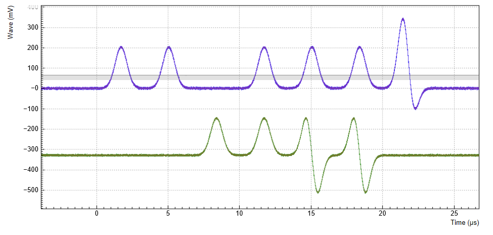
Save and play the Sequencer program with the above settings. The upper plot in Figure 9 shows the AWG signals captured by the Scope. We see the expected Gaussian pulse on AWG Output 1 (green) and the DRAG pulse, which corresponds to the derivative of a Gaussian function, on AWG Output 2.

Figure 9: Dual-channel signal generated by the AWG and captured by the LabOne Scope (dual-channel Scope operation requires UHF-DIG option). The top figure shows two envelope waveforms played in Plain mode, the bottom figure shows the same envelope waveforms played in Amplitude Modulation mode.

While the AWG is running, you can go ahead now and switch both AWG Outputs to Modulation mode. The lower plot in Figure 9 shows the resulting signals, which are the Gaussian and DRAG pulses multiplied by a 5 MHz carrier with phase shift 0° and 90°, respectively.

Table 9: Settings: set both AWG Outputs to Modulation mode
Tab	Sub-tab	Section	#	Label	Setting / Value / State
AWG	Control	Output 1		Mode	Modulation
AWG	Control	Output 2		Mode	Modulation

In this practical case of I/Q modulation, the two AWG Outputs typically require further adjustments of the pulse amplitude, DC offset, and inter-channel phase offset in order to compensate for analog mixer imperfections. All these adjustments can now be done on the fly using the AWG Amplitude, the Signal Output Offset, and the Demodulator Phase settings without having to make any changes to the programmed AWG waveforms.

Stabilizing Carrier-Envelope Offset¶

When playing waveforms in modulation mode, it can sometimes be necessary to synchronize the envelope with the phase of the carrier. This will lead to a final pulse shape that is exactly the same in every repetition. This synchronization is easily achieved with the waitDemodOscPhase command introduced previously. In the following program, we use this command to align the start of the waveform playback with the oscillator phase of demodulator 4, i.e., the carrier phase.

wave w_gauss = gauss(2000, 1000, 200);

while (true) {
  waitDemodOscPhase(4);
  setTrigger(1);
  playWave(1, w_gauss);
  waitWave();
  setTrigger(0);
  wait(100);
}

Look at the generated signal once with and once without the waitDemodOscPhase command. As shown in Figure 10, you will see that with this synchronization command, every generated pulse looks exactly the same.

Figure 10: Amplitude-modulated signal generated by the AWG and captured by the LabOne Scope. The top figure shows repeated waveform without synchronization between carrier and envelope phase. The bottom figure shows the same signal but with synchronization.

Multi-frequency Modulation¶

When the UHF-MF Multi-frequency option is installed, the UHF-AWG supports modulation of multiple carriers with individual envelope signals. Typical use cases are phase cycling protocols in NMR spectroscopy, or frequency-multiplexing techniques. The latter requires the UHF-MF option, whereas the former can be used with the base instrument. Multi-carrier modulation is realized by four-fold interleaving of one AWG channel and individual multiplication of the four channel with one of the demodulator’s oscillator signal. The envelope sampling rate is therefore reduced by a factor of 4, whereas the carrier signal is still generated at the full sampling rate, therefore giving access to the full bandwidth.

With the following sequence program, we generate a series of pulses with changing carrier. The first four pulses each have a single carrier coming from one of the first four oscillators. In the fifth pulse, all carrier signals are superimposed. The interleave command which we use several times allows us to combine four waveforms into one.

const n_samples = 512;
wave w_gauss = 0.25*gauss(n_samples, n_samples/2, n_samples/10);
wave w_zeros = zeros(n_samples);

wave w_channel_1 = interleave(w_gauss, w_zeros, w_zeros, w_zeros);
wave w_channel_2 = interleave(w_zeros, w_gauss, w_zeros, w_zeros);
wave w_channel_3 = interleave(w_zeros, w_zeros, w_gauss, w_zeros);
wave w_channel_4 = interleave(w_zeros, w_zeros, w_zeros, w_gauss);
wave w_all_channels = interleave(w_gauss, w_gauss, w_gauss, w_gauss);

while (true) {
  playWave(w_channel_1);
  playWave(w_channel_2);
  playWave(w_channel_3);
  playWave(w_channel_4);
  setTrigger(1);
  setTrigger(0);
  playWave(w_all_channels);
  playZero(n_samples); //spacing between pulses
}

We need to make further settings in the user interface in order to distribute the AWG signal on the four oscillators. In the Lock-in tab, the outputs of demodulators 1 to 4 need to be enabled. At the same time, we set their output amplitudes to 0 since otherwise a continuous-wave signal would be added. We route the oscillator signals 1 to 4 to the demodulators 1 to 4 by changing the selectors in the Osc column. We set the frequencies of oscillators 1 to 4 to mutually different values. Finally, in the AWG tab we set Modulation to Advanced.

Table 10: Settings: Configure the AWG output and scope trigger
Tab	Sub-tab	Section	#	Label	Setting / Value / State
Scope	Trigger	Trigger		Signal	AWG Trigger 1
Lock-in	All	Oscillators	1	Frequency	5 MHz
Lock-in	All	Oscillators	2	Frequency	10 MHz
Lock-in	All	Oscillators	3	Frequency	20 MHz
Lock-in	All	Oscillators	4	Frequency	40 MHz
Lock-in	All	Demodulators	1	Osc	1
Lock-in	All	Demodulators	2	Osc	2
Lock-in	All	Demodulators	3	Osc	3
Lock-in	All	Demodulators	4	Osc	4
Lock-in	All	Demodulators	8	Phase	0°
Lock-in	All	Output Amplitudes	1-4	Amp 1	0
Lock-in	All	Output Amplitudes	1-4	Enable	ON
AWG	Control	Output 1		Modulation	Advanced

Figure 11 shows the signal captured by the Scope after having made all the settings and uploaded and played the sequence program above.

Figure 11: Amplitude-modulated signal with multiple carriers generated by the AWG and captured by the LabOne Scope.

Signal Output Assignment¶

In addition to the single-channel and dual-channel playback used up to now, there are more options for the channel assignment. The playWave command can be used with different combinations of arguments: with one wave type argument or with two, with a const type integer number specifying the signal output or without. These different combinations of arguments allow the user to independently control the AWG outputs (the digital signal sources inside the instrument) and the place where their signal is routed to (the signal outputs on the front panel). The AWG outputs are represented in the AWG tab, whereas the signal outputs are represented in the In / Out tab and in the Lock-in tab .

The playWave command always assigns the first wave argument to the AWG output 1, and the second one (if it’s provided) to the AWG output 2. Each of the wave arguments can optionally be preceded by an integer argument of type const which specifies the associated signal output. E.g., playWave(2, w_gauss) will play the wave w_gauss on Signal Output 2.

The systematics of channel assignments in the sequence program even works when using multiple instruments. This is discussed in more detail in LabOne Sequence Programming, whereas here we focus on the case of a single UHF instrument. It’s possible to route a single AWG Output to both Signal Outputs at the same time by specifying two integer arguments per wave argument as in playWave(1, 2, w_gauss). This can for example be used to optimize waveform memory. Another option is to add up two AWG Outputs on one Signal Output by using twice the same integer argument as in playWave(1, w_gauss, 1, w_drag). This is e.g. useful in combination with the Modulation Mode as it enables quadrature modulation of an internal oscillator which gives full freedom in controlling the amplitude and phase of a carrier with the AWG. The following sequence program contains a number of examples for these configurations. Figure 12 shows the dual-channel signal generated with this program and measured with the LabOne Scope.

wave w_gauss = 0.5*gauss(8000, 4000, 1000);
wave w_drag  = 0.5*drag(8000, 4000, 1000);

while (true) {
  setTrigger(1);
  // play wave on Signal Output 1 with AWG Output 1 (two equivalent commands):
  playWave(w_gauss);
  playWave(1, w_gauss);
  // play wave on Signal Output 2 with AWG Output 1:
  playWave(2, w_gauss);
  // play identical Wave on Signal Output 1 and 2 generated with AWG Output 1:
  playWave(1, 2,  w_gauss);
  // play independent Waves on Signal Output 1 and 2 generated
  // with AWG Output 1 and 2 (two equivalent commands):
  playWave(w_gauss, w_drag);
  playWave(1, w_gauss, 2, w_drag);
  // add up two independent Waves on Signal Output 1
  // generated with AWG Output 1 and 2:
  playWave(1, w_gauss, 1, w_drag);

  waitWave();
  setTrigger(0);
  wait(10000);
}

Note

Tricky examples are commands like playWave(2, w_gauss) that generate a signal on Signal Output 2, but use the AWG output 1. This means that the relevant Mode and Amplitude (FS) settings are in the section Output 1 of the AWG tab, not in the section Output 2.

Figure 12: Dual-channel signal generated by the AWG and captured by the LabOne Scope (dual-channel Scope operation requires UHF-DIG option). The vertical scales of the two signals have been offset, see

Fast Frequency and Phase Changes¶

The Sequencer of the UHF-AWG is capable of changing all instrument settings. This allows one to change these settings much more quickly and with much more timing precision than when using the graphical user interface or the API. The majority of the settings are made with a delay of less than 100 µs, but the change of oscillator frequency and phase is implemented in a way that changes are made with a delay of less than 150 ns and, even more importantly, with deterministic timing. This is useful e.g. in application fields like NMR spectroscopy or quantum computing, where it’s necessary to make phase or frequency changes rapidly between pulses. Also, this feature allows the user to include special settings that are essential for the correct playback directly in the AWG program.

The instrument settings are made with the setInt or the setDouble commands. Similarly to the corresponding commands used in the LabOne APIs, their arguments are a settings path and a settings value. The quickest way to find the settings path for a given user interface is to use the Command Log feature. Every time a setting is made in the graphical user interface, the corresponding path and value are displayed in the status bar at the bottom of the browser window. For instance, when enabling the Signal Output 1 the displayed path is sigouts/0/enable (zero-based indexing) and the value is 1. A long version of the Command Log can be accessed by clicking on the corresponding button in the status bar. Device Node Tree contains a documentation of all settings paths. In case of using a multi-instrument program, the path has to be prepended with a device number n as in 0/sigouts/0/enable for n=0. The device number corresponds to the order in the Multi Device Sync Tab (n=0 for Leader, n=1 for Follower 1, and so forth).

The following sequence program contains a few examples of settings that are accessible from the AWG. Here we set the AWG channel 1 amplitude to 0.7, and we prepare the Scope by setting its Trigger Source, by enabling the trigger, and by starting the Scope. These settings are examples of "slow" settings, which take of the order of 100 µs to take effect. Subsequently, we play a series of 4 pulses in Modulation mode, and we change the carrier frequency and phase between pulses. These are examples of "fast" settings with a delay of less than 150 ns and deterministic timing. The list of settings that are available for fast real-time access are given in Table 11 along with some additional information.

wave w_gauss = gauss(1024, 512, 100);
const degree_to_phaseshift(const degree) {
  return degree*pow(2, 23)/360.0;
}

const freq_1 = 15e6;
const freq_2 = 35e6;
const phase_1 = degree_to_phaseshift(45);
const phase_2 = degree_to_phaseshift(90);

const set_time = 50;

setDouble('awgs/0/outputs/0/amplitude', 0.7);
setInt('scopes/0/trigchannel', 192); // Set Scope trigger source to AWG Trigger 1
setInt('scopes/0/trigenable', 1);    // Enable Scope trigger
setInt('scopes/0/enable', 1);        // Enable Scope

wait(100000);

while (true) {
  setTrigger(1);
  setTrigger(0);
  playWave(w_gauss);
    waitWave();
    setDouble('oscs/0/freq', freq_1);
    wait(set_time);
  playWave(w_gauss);
    waitWave();
    setDouble('oscs/0/freq', freq_2);
    wait(set_time);
  playWave(w_gauss);
    waitWave();
    setDouble('demods/2/phaseshift', phase_1);
    wait(set_time);
  playWave(w_gauss);
    waitWave();
    setDouble('demods/2/phaseshift', phase_2);
    wait(set_time);
}

Table 11: Settings that are available for fast real-time access from the AWG
Path	Setting	Example
`oscs/0...7/freq`	Oscillator frequency (floating point representation 0-600e6)	`setDouble('oscs/0/freq', 41.23e6);`
`demods/0...7/phaseshift`	Demodulator phase shift (integer 0-8388608 corresponding to 0-360 degrees)	`setInt('demods/3/phaseshift', 1048576);`
`demods/0...7/oscselect`	Demodulator Oscillator selector (integer number 0-7)	`setInt('demods/3/oscselect', 2);`

Combining Signal Generation and Detection¶

The base version of the UHF Arbitrary Waveform Generator contains a single-channel Scope for data acquisition. The UHF hardware platform can furthermore be equipped with a Boxcar Averager, Pulse Counter, or Lock-in Amplifier for more advanced measurement tasks. In this section, we will demonstrate how to use Cross-Domain Triggering and other features in order to combine AWG signal generation and detection in an efficient, precise, and easy way.

Scope/Digitizer¶

Having the Scope/Digitizer in the same housing as the AWG enables internal routing of trigger and marker signals from the AWG to the Scope. The setup of AWG triggers and markers for internal routing is in no way different than for external use and is explained in Generating Triggers with the AWG. Once generated, the generated trigger/marker signals can be selected simply in the Trigger Signal setting of the Scope:

Table 12: Settings: configure Scope for internal triggering by AWG
Tab	Sub-tab	Section	#	Label	Setting / Value / State
Scope	Trigger	Trigger		Signal	AWG Trigger 1

Alternatively, AWG Trigger 2–4 or AWG Marker 1–4 can be used.

Boxcar Averager¶

The Boxcar Tab is an excellent tool for the analysis of signals with low duty cycles. In combination with the AWG, it is well suited whenever the setup response to a short, repeated pulse needs to be measured. Boxcar averager and AWG have to be referenced to the same internal oscillator for proper synchronization. Here, let’s consider the case where the AWG generates a signal on Signal Output 1, and the boxcar unit 1 analyzes the return signal on Signal Input 1. Both the AWG and the Boxcar are referenced to oscillator 1. The following table summarizes the necessary settings.

Table 13: Settings: configure the Boxcar averager and AWG common reference
Tab	Sub-tab	Section	#	Label	Setting / Value / State
Boxcar	Boxcar	Signal Input	1	Osc	1
Boxcar	Boxcar	Signal Input	1	Input Signal	Sig In 1
AWG	Control	Output 1		Mode	Plain
Lock-in	All	Demodulators	1	Osc	1
Lock-in	All	Oscillators	1	Frequency	200 kHz

Synchronization between the AWG and oscillator 1 is achieved with the waitDemodOscPhase used like in the exemplary Sequencer program below. Please refer to Controlling the AWG Repetition Rate for more information.

wave w_gauss = gauss(640, 320, 50);

while (true) {
  waitDemodOscPhase(1);
  playWave(1, w_gauss);
}

Please consider that the duration of the AWG pattern played after the waitPhaseOfDemod command should be shorter than one period of the reference oscillator.

The Periodic Waveform Analyzer (PWA) is a part of the Boxcar averager and usually serves to select a suitable Boxcar integration window. The working principle of the PWA and of the AWG impose some conditions on the repetition frequency. As explained in PWA Averager, the PWA requires a repetition frequency that is incommensurable with the base frequency of 450 MHz in order to faithfully measure a waveform. For the AWG on the contrary, it is preferable to have a repetition rate that is commensurable with the base frequency of 450 MHz, since otherwise the AWG signal jitters by one sequencer period of 4.44 ns.

In choosing between these contradicting requirements, it is usually better to select an repetition frequency that is optimized for a jitter-free AWG signal, i.e., a frequency that is commensurable with 450 MHz. Even though this means that the PWA signal will not look smooth, the Boxcar averager is unaffected by this and performs well. The PWA signal is usually still good enough to help adjusting the Boxcar gate start phase and width. Alternatively, you can use the LabOne Sweeper to vary the Boxcar gate parameters in order to maximize the Boxcar averager signal-to-noise ratio.

Pulse Counter¶

The Pulse Counter Tab supports two run modes that can make use of trigger signals generated by the AWG, gated free running and gated modes. In gated free running mode, the AWG trigger signal defines a pulse counting period by the rising and falling edge of its trigger signal. In gated mode, the AWG trigger signal resets the periodic Pulse Counter timer. Setting up AWG triggers for this purpose is in no way different than for external use and you can follow the explanations in Generating Triggers with the AWG. The following table summarizes the necessary settings in the Counter tab.

Table 14: Settings: configure the Counter gating by the AWG
Tab	Sub-tab	Section	#	Label	Setting / Value / State
Counter	1		1	Gate Input	AWG Trigger 1
Counter	1		1	Mode	Gated Free Running or Gated

Alternatively, AWG Trigger 2–4 can be used as Gate Input.

Lock-in Amplifier¶

The combination of AWG and lock-in amplifier enables a number of fast Sweeper and DAQ measurement modes described in Fast AWG Sweeper Modes and TV Mode Averaging with the Data Acquisition Tool .

Branching and Feed-Forward¶

Using its branching capabilities, the UHFAWG can select the next waveform based on external conditions such as the state of the 32-bit digital input, or internal conditions such as the value of a demodulated signal quadrature.

Branching based on external conditions is typically used in automatic testing in order to allow for fast and flexible control of the AWG playback sequence.
Branching based on internal conditions enables fast feed-forward protocols used for instance in quantum computing.

Inside a Sequencer program, branching is realized with the if statement or with the switch...case statement (cf. LabOne Sequence Programming to learn about the timing difference of the two). In the example below, we read the state of the AWG Analog Trigger Input 1 first, and depending on its state (1 or 0) we play a Gaussian waveform with amplitude 0.5 or 1.0.

wave w_gauss_low  = 0.5 * gauss(8000, 4000, 1000);
wave w_gauss_high = 1.0 * gauss(8000, 4000, 1000);

var trigger_state;
while (true) {
  trigger_state = getAnaTrigger(1);
  if (trigger_state == 0) {
    playWave(1, w_gauss_low);
  } else {
    playWave(1, w_gauss_high);
  }
}

The AWG output depends on how we configure the AWG Analog Trigger Input 1, and what physical signal we provide on that input. The Trigger source may be chosen with the Analog Trigger 1 Signal setting. For a sequence branching application, the Trigger would normally be used in a level-sensitive (as opposed to edge-sensitive) mode, which means that the Rise and Fall checkboxes would be disabled.

In order to set up branching based on external conditions, the Analog Trigger 1 Signal would be set to a physical trigger input, such the Ref / Trigger 2 input. This setting corresponds to a case in which the playback is controlled by an external TTL signal. Much more complex examples can be constructed by using the 32-bit DIO input. This input can be read using the getDIO command that works analogously to the getAnaTrigger command used here.

Branching based on internal conditions is available in the combination of UHF-AWG Arbitrary Waveform Generator with signal detection units such as the UHF-LI Lock-in Amplifier or the UHF-CNT Pulse Counter. In the following we will look into this unique configuration in more detail.

We shall consider the combination of UHFLI and UHF-AWG and realize the situation where a demodulator output signal figures as the AWG Analog Trigger 1 Signal in order to realize a fast feed-forward protocol. This could correspond to a controlled-reset protocol of a quantum bit (qubit), see Phys. Rev. Lett. 109, 240502 (2012). In this protocol, a qubit state is determined in a fast lock-in measurement, and if the measurement yields that the qubit is in an excited state, a reset pulse is applied immediately afterwards. We use the following Sequencer program in order to demonstrate this method.

wave w_gauss_low  = 0.5*gauss(8000, 4000, 1000);
wave w_gauss_high = 1.0*gauss(8000, 4000, 1000);

var trigger_state;
while (true) {
  waitDemodOscPhase(8);
  playWave(1, w_gauss_low);
  waitWave();
  trigger_state = getAnaTrigger(1);
  if (trigger_state == 0) {
    playWave(1, w_gauss_low);
  } else {
    playWave(1, w_gauss_high);
  }

  wait(3000);

  playWave(1, w_gauss_high);
  waitWave();
  trigger_state = getAnaTrigger(1);
  if (trigger_state == 0) {
    playWave(1, w_gauss_low);
  } else {
    playWave(1, w_gauss_high);
  }
}

The program consists of two almost identical blocks enclosed in an infinite while loop. In each block, we first play a Gaussian pulse - let’s call this the measurement pulse. Then we obtain the Analog Trigger 1 state, and then we perform a conditional playback of another Gaussian pulse, let’s call this one the reset pulse.

The two blocks only differ by the amplitude of the measurement pulse: it is either 0.5 or 1.0. This difference can be detected by a fast lock-in measurement. We let the AWG run in Modulation mode using a carrier frequency of 5 MHz, and we configure Demodulator 1 to measure at the same frequency. We set the Demodulator filter time constant to 3 μs, a value that is comparable to the width of the measurement pulse. This means that the demodulator filter roughly integrates the signal over the pulse width.

If we configure the AWG Analog Trigger Input 1 with the appropriate Signal (Demodulator 1 R) and Level (140 mV), the AWG will be able to discriminate the high- and low-amplitude measurement pulses. As a consequence, it will play a low-amplitude reset pulse after a low-amplitude measurement pulse, and a high-amplitude reset pulse after a high-amplitude measurement pulse. Note that the waitWave command ensures that the subsequent command (the getAnaTrigger command which evaluates the measurement value) is executed immediately after (and not during) the playback of the measurement pulse. In our case this is just the right timing to obtain a meaningful demodulator measurement taking into account the demodulator settling time.

The following table summarizes the settings to be made for the feed-forward experiment.

Table 15: Settings: configure the AWG and Demodulators for feed-forward
Tab	Sub-tab	Section	#	Label	Setting / Value / State
AWG	Trigger	Analog Trigger	1	Rise	OFF
AWG	Trigger	Analog Trigger	1	Fall	OFF
AWG	Trigger	Analog Trigger	1	Signal	Demodulator 1 R
AWG	Trigger	Analog Trigger	1	Level	140 mV
AWG	Control	Output	1	Mode	Modulation
Lock-in	All	Low-Pass Filter	1	Order	1
Lock-in	All	Low-Pass Filter	1	TC	3 μs
Lock-in	All	Demodulators	1	Osc	1
Lock-in	All	Demodulators	8	Osc	2
Lock-in	All	Oscillators	1	Frequency	5 MHz
Lock-in	All	Oscillators	2	Frequency	1 kHz
Scope	Trigger	Trigger		Signal	Osc φ Demod 8
Scope	Trigger	Trigger		Enable	ON
Scope	Trigger	Trigger		Run / Stop	ON

Figure 13 shows the signal generated by the AWG in blue. With the UHF-DIG option, we can simultaneously display the R signal of Demodulator 1 in green. The Y2 cursor position shows the AWG Analog Trigger 1 Level of 140 mV. We can observe that the second and the fourth pulse are indeed played conditionally on the demodulator measurement which is evaluated immediately after the measurement pulse has ended. If you adjust the Trigger Level, you will see the live effect on the second and fourth pulse in the signal.

Figure 13: Signal generated by the AWG (blue) and demodulated signal (green; displaying this signal requires UHF-DIG option) captured by the LabOne Scope.

Fast AWG Sweeper Modes¶

The LabOne Sweeper offers special operation modes for fast measurement in combination with the UHF-AWG Arbitrary Waveform Generator. These modes take advantage of the powerful execution control of the LabOne AWG Sequencer and of the high measurement speed of the demodulators. Before using the Sweeper in the special modes, it’s best to first become familiar with its basic operation. This is described in the Sweeper Tab of the Sweeper as well as in the Phase-locked Loop.

Note

For both operation modes described below, the demodulator measurement data rate can be pushed to very high values by gating the demodulator data stream with one of the AWG trigger output channels. Gating is activated using the Trigger setting of the Lock-in tab (collapsed by default). By this method, one can achieve that only the interesting data is transferred to the host PC, but at a much increased peak rate up to 14 MSa/s. This is attractive for applications relying on short and fast measurements interrupted by long dead times.

AWG Index Sweep¶

The Index Sweep mode allows for recording demodulator samples during a rapid pulse sequence played by the AWG. The speed of this mode can be much higher than that of a normal sweep because it has a much smaller overhead time for instrument communication. This is because the Sweeper tool on the host PC takes on a listener role almost all the time. Typically, a fast series of N pulse patterns is played by the AWG, and in each iteration one parameter is changed, e.g. a pulse length, a pulse amplitude, or a pulse delay. For each iteration, the Sweeper records one demodulator sample. The timing of the demodulator measurement relies on one of the AWG Trigger output channels controlled with the AWG setTrigger command. The attribution to a sweep point n=1,...,N relies on the setID(n) command in the AWG sequence program. This command tags the demodulator samples with an identifier number n. The Sweeper listens to the AWG Trigger channel selected in the Sweep Parameter setting. When it receives a trigger, it records a demodulator measurement and attributes it to the sweep point corresponding to the current identifier number. To fine-tune the measurement timing relative to the trigger time, it is advised to configure the settling time in the Settings section of the Sweeper (Advanced Mode).

In the example shown below, we play a Gaussian pulse of width \~1 μs in modulation mode and vary the delay of this pulse relative to a trigger in 1000 steps. We demodulate the signal with demodulator 1 with maximum bandwidth and obtain this data with the Sweeper. As a result, we are able to recover the envelope of the fast pulse in the Sweeper.

In order for the Index Sweep mode to work as desired, the AWG sequence program needs to be compatible with the settings in the Sweeper and in the Lock-in tab. This means the AWG program should contain a for or while loop with a loop count identical to the sweep Length parameter (1000 in this example). The setID needs to be applied inside the loop with the loop count variable as an argument (in the example the count variable is called n). The setTrigger command needs to be applied twice inside the loop: once to set the trigger to the high state, and once to set it back to the low state. The demodulator in use needs to be enabled in the Lock-in tab with a sufficiently high bandwidth compared to the AWG pulse pattern. For this example we set the Filter bandwidth to 5.6 MHz (1^st order) and the demodulator sample rate to 400 kSa/s. Finally, it’s important that the AWG pulse pattern and the demodulator sample rate are compatible: this is easily achieved by using the waitDemodSample command with the demodulator number as an argument (here number 1).

The following file shows an example AWG sequence program in which a pulse is generated with a varying delay relative to the AWG Trigger 1. The pulse is to be played in AWG Modulation mode and measured with demodulator 1.

var sweepPoints = 1000;

// define user utility function
void wait_us(const us) {
  wait(us / 4.444e-3);
}

wave w_gauss = gauss(8000, 4000, 1000);

// define user function
void user_func(var index) {
  // Set ID for assignment to sweep point
  setID(index);
  // Wait to synchronize AWG and demodulator sampling
  waitDemodSample(1);
  // Set Trigger for Sweeper measurement
  setTrigger(1);
  // Wait a variable time (sweep parameter)
  wait(index);
  // Play waveform
  playWave(1, w_gauss);
  waitWave();
  wait_us(3);
  setTrigger(0);
}

// Loop over sweeper variable (waiting time)
var n;
for (n = 0; n < sweepPoints; n = n + 1) {
  user_func(n);
  setID(0);
  wait_us(100);
}
setID(0);

Once a suitable sequence program is loaded, configure the Sweeper for the measurement. Select AWG 1 → Index Sweep Triggers → AWG Trigger 1 as the Sweep Parameter, corresponding to the trigger channel we used in the Sequence program. Set the sweep Length to 1000. In the Sweeper settings sub-tab, set the Filter to Advanced Mode in order to enable "AWG Control". The following table summarizes the settings to be made for this example.

Note

The AWG Index Sweep mode is implicitly enabled when the following two settings are made in the Sweeper: 1) AWG Control is enabled 2) one of AWG Index Trigger 1–4 is selected as the sweep parameter.

Table 16: Settings: configure the AWG and Sweeper for AWG Index Sweep mode
Tab	Sub-tab	Section	#	Label	Setting / Value / State
AWG	Control	Output 1/2		Mode	Modulation
Lock-in	All	Demodulators	1	Enable	ON
Lock-in	All	Demodulators	1	Rate	400 kSa/s
Lock-in	All	Demodulators	1	Low-Pass Filter order	1
Lock-in	All	Demodulators	1	Low-Pass Filter bandwidth	5.6 MHz
Sweeper	Control	Horizontal		Sweep Param	AWG Index Sweep Triggers, Trigger 1
Sweeper	Settings			Filter	Advanced Mode
Sweeper	Settings			BW Mode	Manual
Sweeper	Settings	Statistics		AWG Control	ON
Sweeper	Control			Single	ON

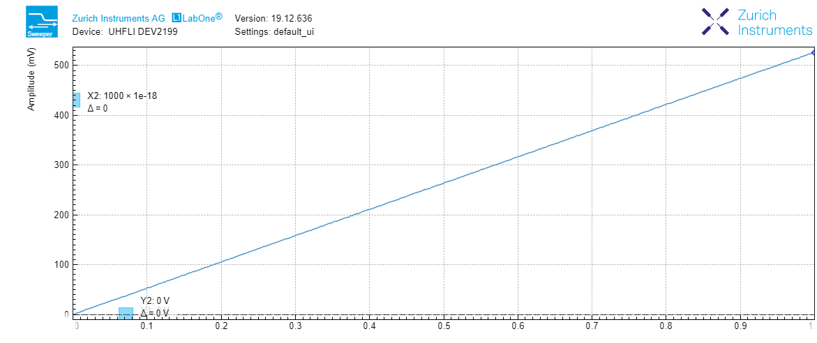
If you start the Sweeper now, it will automatically start the AWG and capture the data very quickly. The result is shown in the following figure.

Figure 14: AWG Index Sweep measurement trace as displayed in the LabOne Sweeper.

AWG Parameter Sweep¶

The AWG Parameter Sweep mode allows for precisely timed demodulator measurements as a function of a large selection of device parameters. This mode combines elements of the basic Sweeper mode and of the AWG Index Sweep mode. Like in the basic Sweeper mode, the Sweeper sets a device parameter (such as an oscillator frequency, an AWG amplitude, or an AWG user register value) and starts measuring the data after that with the possibility to average data for some time. Like in the AWG Index Sweep mode, the precise timing is determined by the AWG Trigger output channel which is controlled with the AWG setTrigger command. When the Sweeper receives a trigger, it starts recording demodulator data for the defined averaging period. To fine-tune the measurement timing relative to the trigger time, it is advised to configure the settling time in the Settings section of the Sweeper (Advanced Mode).

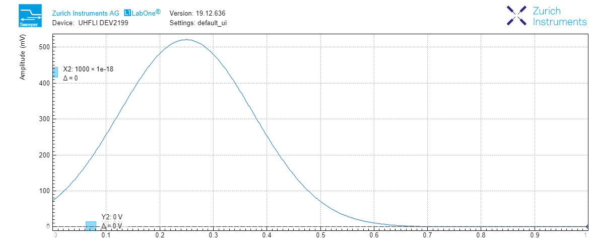
In the example shown here, we play a long pulse in the AWG modulation mode and vary the amplitude of the AWG output with the Sweeper. We demodulate the signal with demodulator 1 with maximum bandwidth and obtain this data with the Sweeper.

For such a measurement, the AWG sequence program should contain two setTrigger commands that define the measurement time: once to set the trigger channel 1 to the high state, and once to set it back to the low state. The demodulator in use needs to be enabled in the Lock-in tab with a sufficiently high bandwidth compared to the AWG pulse pattern speed. Finally, it’s important that the AWG pulse pattern and the demodulator sample rate are compatible: this is easily achieved by using the waitDemodSample command with the demodulator number as an argument (here number 1). The following sequence program is used in this example.

// Play the example at reduced rate of 28 MSa/s
const RATE = AWG_RATE_28MHZ;
const FS = 1.8e9/pow(2, RATE);

// Wait a number of microseconds
void wait_us(const us) {
  wait(1e-6*us*225e6);
}

void user_func() {
  // Total waveform length, 1 ms
  const N = 1e-3*FS;
  // Length of rising edge, 100 us
  const M = 100e-6*FS;
  // Create waveform
  wave edges = blackman(2*M, 1.0, 0.2);
  wave w_pulse = join(cut(edges, 0, M-1),
                      rect(N-2*M, 1.0),
                      cut(edges, M, 2*M-1));
  // Synchronize with demodulator data
  waitDemodSample(1);
  // Start waveform playback
  playWave(1, w_pulse, RATE);
}

// Function for enabling sweeper recording, from/to in microseconds
void sweeper_record(const from_us, const to_us) {
  // Wait a bit, then make sweeper record data
  wait_us(from_us);
  setTrigger(1);
  wait_us(to_us-from_us);
  setTrigger(0);
}

// Execute the subprograms
user_func();
sweeper_record(100, 900);

Note

The AWG Parameter Sweep mode is implicitly enabled when the following two settings are made in the Sweeper: 1) AWG Control is enabled 2) the sweep parameter is anything except AWG Index Trigger 1–4.

The following table summarizes the settings to be made for this example.

Table 17: Settings: configure the AWG and Sweeper for AWG Parameter Sweep mode
Tab	Sub-tab	Section	#	Label	Setting / Value / State
AWG	Control	Output 1/2		Mode	Modulation
Lock-in	All	Demodulators	1	Enable	ON
Lock-in	All	Demodulators	1	Rate	400 kSa/s
Lock-in	All	Demodulators	1	Low-Pass Filter order	1
Lock-in	All	Demodulators	1	Low-Pass Filter bandwidth	5.6 MHz
Sweeper	Control	Horizontal		Sweep Param	AWG Output 1 Amplitude
Sweeper	Settings			Filter	Advanced Mode
Sweeper	Settings			BW Mode	Manual
Sweeper	Settings	Statistics		AWG Control	ON
Sweeper	Control			Single	ON

If you start the Sweeper now, it will automatically start the AWG and capture the data very quickly. The result is shown in the following figure.

Figure 15: AWG parameter sweep measurement trace as displayed in the LabOne Sweeper.

TV Mode Averaging with the Data Acquisition Tool¶

The LabOne Data Acquisition (DAQ) tool in combination with the UHF-AWG offers a special cyclic data acquisition and averaging also known as TV mode averaging. This can be used to realize drift-resistant measurements as a function of pulse parameters such as pulse width, amplitude, or carrier frequency. One classic example is the measurement of Rabi oscillations of a quantum bit (qubit). In this section, we’ll explain the Data Acquisition tool cyclic averaging using an example inspired by the Rabi oscillation measurement. Since it’s not that easy to simulate the behavior of a qubit in a table-top experiment, the example doesn’t correspond exactly to a real pulse pattern, but it is intended to demonstrate the typical signal generation and acquisition tasks that occur in an actual experiment, and to produce a data set that resembles that of an actual experiment.

In the example, we’ll make use of the following features:

Data Acquisition tool Grid Mode to capture 2D data sets
UHF-AWG data tagging for 2D data row assignment
UHF-AWG indexed waveform playback
Demodulator gated data streaming for highest peak data rates

The following file shows the AWG sequence program for the Rabi example. Copy and upload this program to the AWG or select it from the examples drop-down menu.

const rows = 100;      // number of different pulse amplitudes
const f_s = 1.8e9;     // AWG sampling rate
const f_seq = 225e6;   // sequencer clock frequency
const pulse_width_sec = 100e-9; // width of the Gaussian pulse (s)
const gate_window_sec = 1.5e-6; // width of the demodulator data gating window (s)
const period_sec = 30e-6; // time between successive pulses (s)

void gate_start() {
  setTrigger(0b01); // activate gate signal (AWG Trigger 1)
  wait(20);         // wait a certain time (at least the inverse of the
                    // demodulator sample rate) to make the rising edge
                    // of AWG Trigger 2 visible in the demodulator data stream
  setTrigger(0b11); // activate trigger signal for Data Acquisition tool (AWG Trigger 2)
}

void gate_stop() {
  setTrigger(0b00); // reset gate and trigger signal
}

const gate_window = gate_window_sec*f_seq;

// Waveform generation
const pulse_width = pulse_width_sec*f_s;
const waveform_length = 7*pulse_width_sec*f_s;

cvar i;
cvar amplitude;
const decay_time = 100;
const rabi_period = 40;
wave w_array;
for (i=0; i<rows; i=i+1) {
  amplitude = 0.5 + exp(-i/decay_time)*0.5*cos(2*M_PI*i/rabi_period);
  wave w_segment = amplitude*gauss(waveform_length, waveform_length/2, pulse_width);
  w_array = join(w_array, w_segment);
}

// Beginning of the core sequencer program executed on the UHF at run time
var t;
var id = 0; // Row ID to be used by the Data Acquisition tool for data triage
const loop_end = rows*waveform_length;
while (true) {
  id = 0;
  for (t = 0; t < loop_end; t = t+waveform_length) {
    setID(id);          // set the row ID
    wait(period_sec*f_seq);
    waitDemodSample(1); // synchronize the AWG with the demodulator sample rate
    playWaveIndexed(w_array, t, waveform_length); // play waveform segment
    wait(200);
    gate_start();       // start the demodulator gate signal
    wait(gate_window);
    gate_stop();        // stop the demodulator gate signal
    id = id+1;          // increment row ID
  }
}

In the first part of the program, we define two user functions gate_start() and gate_stop() which allow us to define a demodulator gating window using the AWG Trigger 1. Inside the gating window defined by AWG Trigger 1, we place a rising edge of AWG Trigger 2. The latter figures as a trigger signal for the Data Acquisition tool.

In the second part of the program, we use a for loop to define an array of pulse shapes that we intend to play back cyclically in the sequence program. The number of pulses is controlled using the constant rows which we set to 100. All 100 pulse waveforms have a Gaussian shape with different amplitudes. We combine all these 100 pulse shapes into one long waveform called w_array which we are going to access in a segmented manner during the playback. By using only cvar (compile-type variable) data types, we ensure that this loop is evaluated at compile time.

In the third part of the program, we define the waveform playback and other instructions to be executed at run time. The program features a for loop over rows iterations. At the beginning of each iteration, we use the setID command to tag the demodulator data with the row number i. This index will be read by the Data Acquisition tool to assign its data to the correct row. After the setID command and some waiting and synchronization time, we start the segmented waveform playback using the playWaveIndexed command. By using the run-time variable t as a sample index, we access one segment of the long waveform w_array that corresponds to one of the 100 pulses. After the start of the waveform playback, we use the gate_start and gate_stop functions to define a gate window of about 1.5 µs width for the measurement.

In the Lock-in tab, we configure demodulator 1 for fast measurements. We first set the demodulator 1 Trigger from Continuous to AWG Trigger 1 and the Trig Mode to High (the Trigger section to the right of the Demodulator section is collapsed by default). Because now the demodulator will only stream data during the short windows when the AWG Trigger is high, we can in turn increase its data rate to the maximum of 14 MSa/s without reaching a limitation by the interface. We also set the measurement bandwidth to the maximum of 5.6 MHz (1^st-order filter).

In the DAQ tab tab (Settings sub-tab), we first set the Hold Off and Delay both to 0 s. We set Trigger Signal to AWG Trigger 2. In the Grid sub-tab, we enable the Grid Mode by setting Mode to Linear. In this mode, the Data Acquisition tool will resample the data on the horizontal axis using linear interpolation to a number of samples defined by the Columns settings. We can set the Columns to 200 and the Duration to 2 µs. In this way, we cover optimally the short pulses generated by the AWG. The Rows setting has to match the number of different pulse shapes defined by the constant rows in the AWG program. By enabling AWG Control, we tell the Data Acquisition tool to assign each shot of data to the row corresponding to the AWG tag setID on the data. By using the Average operation, and a certain number of repetitions, e.g. 10, we obtain a 2D data set averaged over several full periods of the experiment. To display this set using a color scale graph, set Plot Type to 2D.

All necessary settings are summarized in Table 18. Once these settings are made, we can start the Data Acquisition tool and subsequently the AWG using the "Single" buttons. The Data Acquisition tool should then capture and display a graph such as the one shown in Figure 16. In this graph, the horizontal axis corresponds to the time dependence given by the Gaussian pulse shape. The vertical axis shows the row number 1...100 which corresponds to the pulse parameter varied in the experiment. In this example, we artificially generated pulses with an exponentially decaying, oscillating amplitude similar to what would be seen in a Rabi oscillation experiment.

Table 18: Settings: configure the AWG and Data Acquisition tool
Tab	Sub-tab	Section	#	Label	Setting / Value / State
AWG	Control	Output 1/2		Mode	Modulation
Lock-in	All	Demodulators	1	Enable	ON
Lock-in	All	Demodulators	1	Trigger	AWG Trigger 1
Lock-in	All	Demodulators	1	Trig Mode	High
Lock-in	All	Demodulators	1	Enable	ON
Lock-in	All	Demodulators	1	Rate	14 MSa/s
Lock-in	All	Demodulators	1	Low-Pass Filter order	1
Lock-in	All	Demodulators	1	Low-Pass Filter bandwidth	5.6 MHz
Lock-in	All	Signal Outputs		Signal Output 1	ON
DAQ	Settings	Trigger Settings		Trigger Signal	AWG Trigger 2
DAQ	Settings	Horizontal		Hold Off Time	0 s
DAQ	Settings	Horizontal		Delay	0 s
DAQ	Grid	Grid Settings		Mode	Linear
DAQ	Grid	Grid Settings		Operation	Average
DAQ	Grid	Grid Settings		Duration	2 µs
DAQ	Grid	Grid Settings		Columns	200
DAQ	Grid	Grid Settings		Rows	100
DAQ	Grid	Grid Settings		Repetitions	10
DAQ	Grid	Grid Settings		AWG Control	ON
DAQ	Grid	Display		Plot Type	2D

Figure 16: 2D data captured with the Data Acquisition tool in Grid Mode. The horizontal axis shows the time, the vertical axis is the row number, and the color scale shows the demodulator amplitude.

Four-channel Aux Output¶

For applications requiring more channels and/or higher voltages, the UHF-AWG can generate signals on the auxiliary outputs of the UHF instrument. To this end the AWG resources for one fast channel (1.8 GSa/s) can be reallocated so as to generate four independent signals at 14 MSa/s and 16 bit resolution in a ±10 V range.

In the sequence program, the functionality is available through the playAuxWave function. The function requires four waveforms of equal length as arguments.

We configure the multi-purpose Auxiliary Outputs for AWG signal generation by setting the Auxiliary Output Signal to AWG in the Auxiliary tab. Each Auxiliary Output corresponds to one of the four rows in the tab. The Channel setting allows you to route one of the four AWG Outputs (the four waveforms of the playAuxWave command) to the given Auxiliary Output. Typically for the first row the Channel is set to 1, for the second row to 2, and so forth.

We intend to monitor the individual Auxiliary signals with the Scope on Signal Input 1. Before making the corresponding BNC connections, it’s good practice to adjust the Auxiliary Output Lower and Upper Limits in order to prevent damage to the Signal Input. You can use the Scale and the Offset setting in order to modify the signal.

The Auxiliary Outputs have a much lower analog bandwidth than the Signal Outputs. It is therefore necessary to work at a sampling rate of 14 MSa/s or less. In order to combine slow Auxiliary Output signals with fast signals on the Signal Outputs, it’s useful to set the sampling rate for every individual waveform play command. In the following example, we first play four waveforms in parallel on the Auxiliary Outputs at reduced sampling rate, and then one waveform on the Signal Output 2 at full sampling rate.

// Sampling rate of the system, adjust accordingly if the rate is reduced
const FS = 1800e6;
// Frequency of the 'sine' in the SINC waveform
const F_SINC = 42e6;

// Generate the four-channel auxiliary output waveform
wave aux_ch1 =  1.0*gauss(8000, 4000, 1000);
wave aux_ch2 =  0.5*gauss(8000, 4000, 1000);
wave aux_ch3 = -0.5*gauss(8000, 4000, 1000);
wave aux_ch4 = -1.0*gauss(8000, 4000, 1000);

// Generate a waveform to be played on Signal Output 2
wave w_sinc = sinc(8000, 4000, FS/F_SINC);

while (true) {
  // play the four Aux Output channels at reduced rate
  playAuxWave(aux_ch1, aux_ch2, aux_ch3, aux_ch4, AWG_RATE_14MHZ);
  // play a wave on Signal Output 2
  playWave(w_sinc, AWG_RATE_1800MHZ);
}

The following table summarizes the settings to be made for this example.

Table 19: Settings: configure the AWG for generating signals on the Auxiliary Outputs
Tab	Sub-tab	Section	#	Label	Setting / Value / State
AWG	Control	Output 1/2		Mode	Plain
Auxiliary		Aux Output	1-4	Lower/Upper Limit	–1.5 V/+1.5 V
Auxiliary		Aux Output	1-4	Signal	AWG
Auxiliary		Aux Output	1	Channel	1
Auxiliary		Aux Output	2	Channel	2
Auxiliary		Aux Output	3	Channel	3
Auxiliary		Aux Output	4	Channel	4

Note

The four-channel AWG mode features a sample hold functionality: the output voltage of the last sample of a waveform remains fixed after the waveform playback is over. This can be used to control the output voltage between pulses.

Debugging Sequencer Programs¶

When generating fast signals and observing them with the LabOne Scope, in some configurations you may observe timing jitter or unexpected delays in the generated signal. There are two main reasons for that. The first reason is linked to the AWG’s memory architecture, which is based on a main memory and a cache memory. Waveform data stored in the main memory (128 MSa per channel) must be copied to the cache memory (32 kSa per channel) prior to playback. The bandwidth available for this data transfer is less than that required by the AWG for dual-channel operation at 1.8 GSa/s. Therefore, if the AWG is configured to play waveforms longer than what fits in the cache memory in dual-channel mode at 1.8 GSa/s, interruptions in the generated signal may be observed. The second reason is connected to the AWG compiler concept explained in Description. When a program in the Sequence Editor is compiled into machine code that can be executed by the Sequencer hardware, single lines of code may be expanded into several machine instructions. Each instruction requires one clock cycle (4.44 ns) for execution. Therefore, the final timing of the generated waveform may not always be completely apart from looking solely at the high-level sequencer program. The compiled program, which defines the actual timing, is displayed in the Advanced sub-tab.

Please take the following tips into consideration when operating the UHF-AWG. They should help you prevent and solve timing problems.

The Scope and the AWG share the same memory, which means that operating them together at high sampling rates affects the performance of both of them. Note that this is only a concern when the AWG is playing back waveforms that are too large to fit in the cache memory. If this is the case it may prove difficult to visualize the generated AWG signal using the LabOne Scope. One option for visualizing such long waveforms is to reduce the sampling rate of both the AWG and the Scope to 225 MHz, which allows both the AWG and the Scope to operate in dual-channel mode simultaneously. The overall shape of the generate AWG signal can then be visualized and evaluated. The sampling rate of the AWG can then be increased once you are satisfied with the shape of the generated signals.
Minimize waveform memory (1): use the possibility to vary the sample rate during playback. The playWave command (and related commands) accept a sampling rate parameter, which means slow and fast signal components can be played at different rates.
Minimize waveform memory (2): take advantage of the amplitude modulation mode in order to generate signals at the full bandwidth, but with reduced envelope sampling rate.
Minimize waveform memory (3): in four-channel (Auxiliary Output) mode, the signal amplitude of the last sample after a waveform playback is held. This eliminates the need for long waveforms with constant amplitude, e.g. on a pulse plateau.
Check the occupied waveform cache memory in the Waveform sub-tab. If you stay below 100%, the performance is best and there is no interference with the LabOne Scope.
Take advantage of the AWG state signals available on the Trigger outputs. In the DIO tab you can select from a number of options for outputting the AWG state as TTL signals, such as "fetching", or "playing". Monitoring these signals on a scope can help in understanding the AWG timing.
When possible, use the repeat loop instead of the for and while loops. The for and while loops evaluate and compare run-time variables, which makes them slower to execute in comparison to the repeat loop.
Fill up sequencer waiting time with useful commands. Placing commands and run-time variable operations just before a wait command (and related commands) in the sequence program means they will be executed when the sequencer has time.
When you need sample-precise timing between analog and digital output signals, use the AWG Markers rather than the AWG Triggers or the DIO outputs.
When using the four-channel Auxiliary Output mode, be aware that the timing between Signal Output and Aux outputs is not well-defined. Use a scope to adjust inter-channel delays.
Be aware that the sequencer instruction memory is also segmented into a cache memory and main memory. Very long sequence programs therefore require fetching operations, which costs some time. You can read the memory usage in the Advanced sub-tab.