Scope Tab
The Scope is a powerful time domain and frequency domain measurement tool as introduced in Unique Set of Analysis Tools and is available on all UHF Series instruments.
Features
- One input channel with 64 kSa of memory; upgradable to two channels with 128 MSa memory per channel (UHF-DIG option)
- 12 bit nominal resolution
- Simultaneous display of both input channels with up to 1.8 GSa/s (requires UHF-DIG option)
- Segmented recording (requires UHF-DIG option)
- Colorscale display for imaging (requires UHF-DIG option)
- Fast Fourier Transform (FFT): up to 900 MHz span, spectral density and power conversion, choice of window functions
- Sampling rates from 27 kSa/s to 1.8 GSa/s; up to 36 μs acquisition time at 1.8 GSa/s or 2.3 s at 27 kSa/s
- 8 signal sources including Signal Inputs and Trigger Inputs; up to 8 trigger sources and 2 trigger methods
- Independent hold-off, hysteresis, pre-trigger and trigger level settings `
- Support for Input Scaling and Input Units
- Continuous recording of both input channels at up to 7 MSa/s over USB and 14 MSa/s over 1GbE
Description
The Scope tab serves as the graphical display for time domain data. Whenever the tab is closed or an additional one of the same type is needed, clicking the following icon will open a new instance of the tab.
| Control/Tool | Option/Range | Description |
|---|---|---|
| Scope | Displays shots of data samples in time and frequency domain (FFT) representation. |
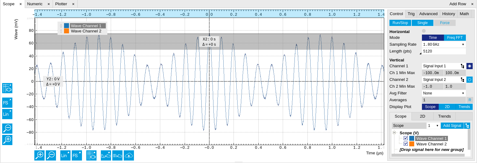
The Scope tab consists of a plot section on the left and a configuration section on the right. The configuration section is further divided into a number of sub-tabs. It gives access to a single-channel oscilloscope that can be used to monitor a choice of signals in the time or frequency domain. Hence the X axis of the plot area is time (for time domain display, Figure 1) or frequency (for frequency domain display, Figure 3). It is possible to display the time trace and the associated FFT simultaneously by opening a second instance of the Scope tab. The Y axis displays the selected signal that can be modified and scaled using the arbitrary input unit feature found in the Lock-in tab.
The Scope records data from a single channel at up to 1.8 GSa/s. The channel can be selected among the two Signal Inputs, Auxiliary Inputs, Trigger Inputs and Demodulator Oscillator Phase. The Scope records data sets of up to 64 kSa samples in the standard configuration, which corresponds to an acquisition time of 36 μs at the highest sampling rate. The performance of the Scope is comparable to that of entry-level GHz sampling rate oscilloscopes. The Scope may be upgraded with the UHF-DIG Digitizer option, which enables two channels to be recorded in parallel, increases the available memory to 128 MSa/channel, and allows recording and color scale display of data in a segmented fashion. The UHF-DIG Digitizer option also enables a continuous recording mode with a sampling rate of up to 28 MSa/s.
The product of the inverse sampling rate and the number of acquired points (Length) determines the total recording time for each shot. Hence, longer time intervals can be captured by reducing the sampling rate. The Scope can perform sampling rate reduction either using decimation or BW Limitation as illustrated in Figure 2. BW Limitation is activated by default, but it can be deactivated in the Advanced sub-tab. The figure shows an example of an input signal at the top, followed by the Scope output when the highest sample rate of 1.8 GSa/s is used. The next signal shows the Scope output when a rate reduction by a factor of 4 (i.e. 450 MSa/s) is configured and the rate reduction method of decimation is used. For decimation, a rate reduction by a factor of N is performed by only keeping every Nth sample and discarding the rest. The advantage of this method is its simplicity, but the disadvantage is that the signal is undersampled because the input filter bandwidth of the UHF Series instrument is fixed at 600 MHz. As a consequence, the Nyquist sampling criterion is no longer satisfied and aliasing effects may be observed. The default rate reduction mechanism of BW Limitation is illustrated by the lowermost signal in the figure. BW Limitation means that for a rate reduction by a factor of N, each sample produced by the Scope is computed as the average of N samples acquired at the maximum sampling rate. The effective signal bandwidth is thereby reduced and aliasing effects are largely suppressed. As can be seen from the figure, with a rate reduction by a factor of 4, every output sample is simply computed as the average of 4 consecutive samples acquired at 1.8 GSa/s.

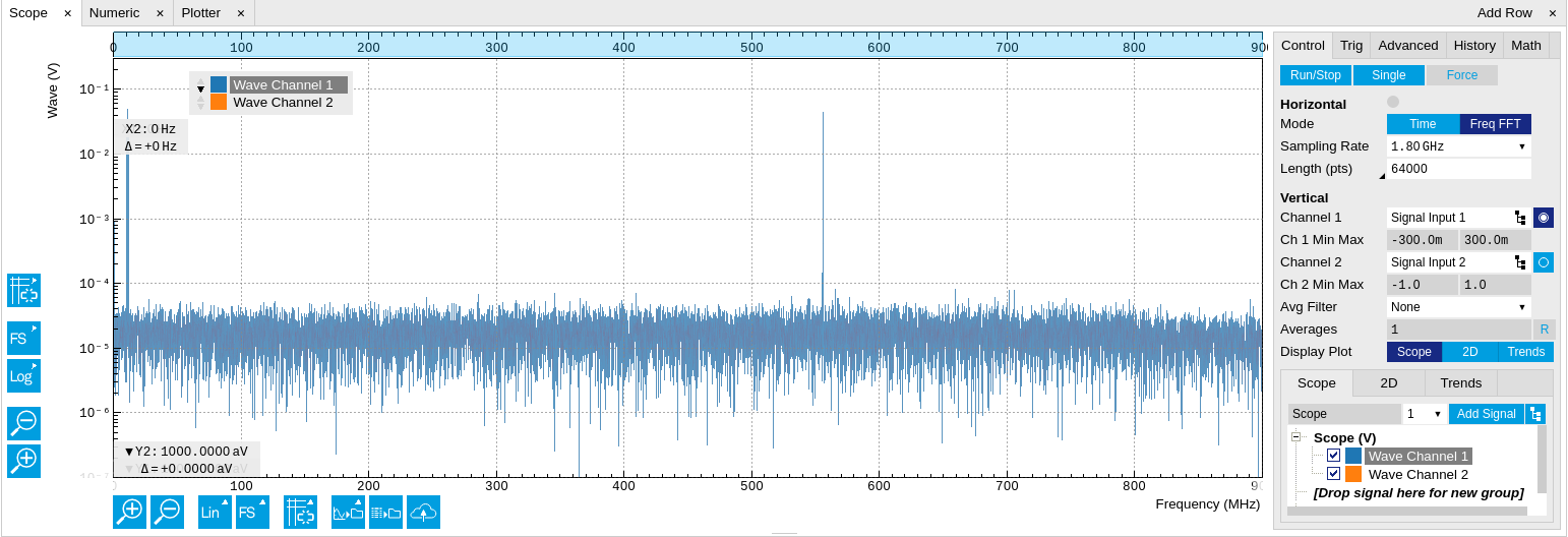
The frequency domain representation is activated in the Control sub-tab by selecting Freq Domain FFT as the Horizontal Mode. It allows the user to observe the spectrum of the acquired shots of samples. All controls and settings are shared between the time domain and frequency domain representations.
The Scope supports averaging over multiple shots. The functionality is implemented by means of an exponential moving average filter with configurable filter depth. Averaging helps to suppress noise components that are uncorrelated with the main signal. It is particularly useful in combination with the Frequency Domain FFT mode where it can help to reveal harmonic signals and disturbances that might otherwise be hidden below the noise floor.
The Trigger sub-tab offers all the controls necessary for triggering on different signal sources. When the trigger is enabled, then oscilloscope shots are acquired whenever the trigger conditions are met. Trigger and Hysteresis levels can be indicated graphically in the plot. A disabled trigger is equivalent to continuous oscilloscope shot acquisition.
Digitizer upgrade option
The UHF-DIG Digitizer option greatly enhances the performance of the Scope with the addition of the following features
- Simultaneous recording of two Scope channels
- Memory depth of 128 MSa for both Scope channels
- Additional input signal sources (Boxcar, Demodulator, Arithmetic Unit and PID data)
- Segmented recording
- Imaging support with colorscale display
- XY display of two channels
- Trigger gating
- Additional trigger input sources that allow for cross-domain triggering
- Additional trigger/marker output sources based on the state of the Scope
- Continuous scope data streaming
This additional functionality can be enabled on any UHF Series instrument with an option key. Please contact Zurich Instruments to get more information. The following sections explain the Digitizer features in more detail.
Two channels and extended memory depth
The UHF-DIG option enables simultaneous dual-channel recording. This allows for very exact relative timing measurements. With the XY display, it’s possible to plot two signals against each other, e.g. for quick visualization of phase offsets or characteristic curves. Each channel can be assigned a different signal source. Trigger settings, sampling rate, and recording length settings are shared between both channels. An increased shot length of up to 128 MSa compared to the standard 64 kSa allows for longer recording times and FFTs with finer frequency resolution for the same frequency span.
Additional input sources
Besides the Signal Input, Trigger Input, Auxiliary Input, and Oscillator Phase the UHF-DIG option also allows for recording of Demodulator, PID, Boxcar and Arithmetic Unit signals. This functionality is very powerful in that it allows short bursts to be recorded with very high sampling rates. In order to optimally use the vertical resolution, the upper and lower limit of these input signals should be chosen appropriately. Before sampling, a scaling and an offset are applied to the input signal in order to get 12 bit resolution between the lower and upper limit. The applied scaling and offset values are transferred together with the scope data, which allows for recovery of the original physical signal strength in absolute values. For directly sampled input signals like the Signal Inputs or Trigger Inputs, the limits are read-only values and reflect the selected input range.
Segmented data recording and imaging
The segmented data recording mode allows for a significant reduction of the hold-off time between scope shots to less than 100 μs. This is achieved by intermediate storage of a burst of up to 32768 scope shots, called segments, in the instrument memory. In this way, the Scope does not have to wait after each shot until the data transfer to the host computer is completed. In segmented data recording mode, the Scope provides a two-dimensional color scale display of the data particularly useful for imaging applications. When used over the API, the data of each shot will contain information on the segment number.
Trigger gating
With the UHF-DIG option installed the user can make full use of the Trigger Engine. If trigger gating is enabled, a trigger event will only be accepted if the gating input is active.
Additional trigger input sources
By using a Demodulator , PID, Boxcar, or Arithmetic Unit signal as trigger source, the Scope can be used in a cross-domain triggering mode. This allows, for example, for time domain signals to be recorded in a synchronous fashion triggered by the result from analyzing a signal in the frequency domain by means of a demodulator.
Note
Choose a negative delay (pre-trigger) to compensate for the delay of the Demodulator, PID, Boxcar or Arithmetic Unit.
Continuous Scope data streaming
Normal scope operation records scope shots into the instrument memory. This allows for recording of up to 1.8 GSa/s until the memory is full. After each scope shot there will be a dead time, also known as hold-off time, to re-arm the trigger, address the next memory block and transfer the data to the PC. Due to this dead time scope shots cannot be recorded back to back. In order to record very long scope shots (digitizer mode) the Scope data can be streamed directly to the host computer bypassing the instrument memory. This allows for continuous recording of very long Scope traces that exceed the available memory depth of the instrument. The streamed Scope data is available for display in the Plotter tab together with all other streaming data. Due to the limited transfer bandwidth over the TCPIP or USB interface, the maximum sampling rate is smaller than for shot operation. The sampling rate for the Scope streaming channels and the enabling of each channel is controlled in the Advanced sub-tab of the Scope. As the sampling rate of the Scope streaming can be adjusted independently from the Scope shot sampling rate it is possible to record continuous data together with triggered high sampling rate Scope shots.
Scope state output on Trigger Output
The UHF-DIG option extends the list of available Trigger Outputs by the six elements: Scope Trigger, Scope Armed, Scope Active and their logically inverse signals. The Trigger Output signals are controlled on the DIO tab (DIO Tab). Figure 4 shows an illustration of the signal that will be generated on the Trigger Output when one of the six new Scope-related sources is selected. An example input signal is shown at the top of the figure. It is assumed that the Scope is configured to trigger on this input signal on a rising edge crossing the level indicated by the stippled line.
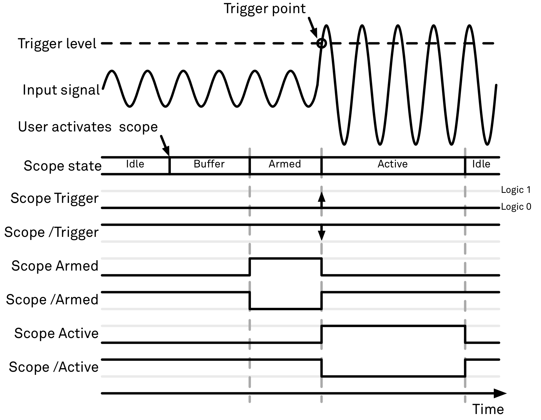
The Scope can be thought of as having a state, which changes over time. The state is shown below the input signal in the figure. When the Scope is completely inactive, it is said to be in the Idle state. When the user then activates the Scope, it will transition into a Buffer state. In this state the Scope will start to record the input signal. It will remain in this state until sufficient data has been recorded to fulfill the user requirement for recording data prior to the trigger point as controlled by the trigger Reference and Delay fields in the user interface. Once sufficient data has been recorded, the Scope will transition to the Armed state. In this state the Scope is ready to accept the trigger signal. Note that the Scope will continue to record data for as long as it is in the Armed state, and that if no trigger is defined, the Scope will simply pass straight through the Armed state. Once the input signal passes the Trigger level the Scope will trigger, and at the same time its state will change from Armed to Active. The Scope will remain in the Active state, where it also records data, until sufficient data has been recorded to fulfill the Length requirement configured in the user interface. Once enough data has been acquired, the Scope will transition back into the Idle state where it will wait for the time configured with the Hold-off time before it either starts the next measurement automatically (in case Run is active) or waits for the user to reactivate it.
The trigger source selector allows information about the Scope state to be reproduced on the Trigger Output in a number of ways. The signal that will appear on the output is shown with the six bottommost traces in the figure. Note that these traces are shown as digital signals with symbolic values of logic 0 and 1. These values will of course be actual voltages when measured on the device itself.
First, if Scope Trigger is selected then the trigger output will have a signal that is asserted, which means that it goes high, when the scope triggers, i.e. changes from the Armed to the Active state. The signal will normally have a very short duration and, therefore, it is shown with an arrow in the figure. The duration can be increased by means of the Width input field, which can be found next to the Output Signal selector on the DIO tab. If Scope/Trigger is selected, then the same signal will appear on the output, but it will simply be inverted logically.
Next, if the Scope Armed source is selected, the trigger output will be asserted as long as the Scope is in the Armed state. Again, this means that the Scope has recorded enough data to proceed with the acquisition and is waiting for the trigger condition to become satisfied. In this example, since a rising edge trigger is defined, the trigger condition becomes satisfied when the input signal goes from below the trigger level to above the trigger level.
Similarly, if Scope /Armed is selected, the trigger output will be asserted (i.e. at logic 1) whenever the Scope is in a state different from the Armed state. The same explanation holds for the remaining two configuration options, except here the trigger output is asserted when the Scope is in the Active state or when it is not in the Active state.
Functional Elements
| Control/Tool | Option/Range | Description |
|---|---|---|
| Run/Stop |  |
Runs the scope/FFT continuously. |
| Single |  |
Acquires a single shot of samples. |
| Force |  |
Force a trigger event. |
| Mode | Freq Domain (FFT) | Switches between time and frequency domain display. |
| Time Domain | ||
| Sampling Rate | 27.5 kSa/s to 1.8 GSa/s | Defines the sampling rate of the scope. The numeric values are rounded for display purposes. The exact values are equal to the base sampling rate divided by 2^n, where n is an integer. |
| Length Mode | Switches between length and duration display. | |
| Length (pts) | The scope shot length is defined in number of samples. The duration is given by the number of samples divided by the sampling rate. The UHF-DIG option greatly increases the available length. | |
| Duration (s) | The scope shot length is defined as a duration. The number of samples is given by the duration times the sampling rate. | |
| Length (pts) or Duration (s) | numeric value | Defines the length of the recorded scope shot. Use the Length Mode to switch between length and duration display. |
| Channel 1/2 |  |
Selects the signal source for the corresponding scope channel. Navigate through the tree view that appears and click on the required signal. Note: Channel 2 requires the DIG option. |
| Min | numeric value | Lower limit of the scope full scale range. For demodulator, PID, Boxcar, and AU signals the limit should be adjusted so that the signal covers the specified range to achieve optimal resolution. |
| Max | numeric value | Upper limit of the scope full scale range. For demodulator, PID, Boxcar, and AU signals the limit should be adjusted so that the signal covers the specified range to achieve optimal resolution. |
| Enable | ON / OFF | Activates the display of the corresponding scope channel. Note: Channel 2 requires the DIG option. |
| Average Filter | Enable averaging filter which obtains and displays the average of scope shots continuously. Depending on the Scope Mode, the source data for averaging is either the Time or the FreqFFT trace. | |
| Off | Averaging is turned off. | |
| On | Consecutive scope shots are averaged and the outcome is displayed. | |
| Weight | integer value | Define the weight function for exponential averaging which corresponds to the number of scope shots required to reach 63% settling. Twice the number of shots yields 86% settling. The improvement in resolution is limited by the square root of the weight parameter. |
| Averages | integer value | The number of shots to average on the device before returning the data. |
| Reset |  |
Reset the averaging filter. |
| Averaging Method | Select the averaging method between Uniform and Exponential. | |
| Exponential | Apply exponential weight on the scope shots while averaging. | |
| Uniform | Apply uniform weight on the scope shots while averaging. | |
| Count | integer value | Displays the number of scope shots that have been averaged. |
For the Vertical Axis Groups, please see the table "Vertical Axis Groups description" in the section called "Vertical Axis Groups".
| Control/Tool | Option/Range | Description |
|---|---|---|
| Trigger | grey/green/yellow | When flashing, indicates that new scope shots are being captured and displayed in the plot area. The Trigger must not necessarily be enabled for this indicator to flash. A disabled trigger is equivalent to continuous acquisition. Scope shots with data loss are indicated by yellow. Such an invalid scope shot is not processed. |
| Enable | ON / OFF | When triggering is enabled scope data are acquired every time the defined trigger condition is met. If disabled, scope shots are acquired continuously. |
| Signal | |
Selects the trigger source signal. Navigate through the tree view that appears and click on the required signal. |
| Slope Rise | Triggers when the trigger signal is crossing the trigger level from low to high. | |
| Slope Fall | Triggers when the trigger signal is crossing the trigger level from high to low. | |
| Level (V) | trigger signal range (negative values permitted) | Defines the trigger level. |
| Hysteresis Mode | Selects the mode to define the hysteresis strength. The relative mode will work best over the full input range as long as the analog input signal does not suffer from excessive noise. | |
| Hysteresis (V) | Selects absolute hysteresis. | |
| Hysteresis (%) | Selects a hysteresis relative to the adjusted full scale signal input range. | |
| Hysteresis (V) | trigger signal range (positive values only) | Defines the voltage the source signal must deviate from the trigger level before the trigger is rearmed again. Set to 0 to turn it off. The sign is defined by the Edge setting. |
| Hysteresis (%) | numeric percentage value (positive values only) | Hysteresis relative to the adjusted full scale signal input range. A hysteresis value larger than 100% is allowed. |
| Show Level | ON / OFF | If enabled shows the trigger level as grey line in the plot. The hysteresis is indicated by a grey box. The trigger level can be adjusted by drag and drop of the grey line. |
| Trigger Gating | Select the signal source used for trigger gating if gating is enabled. This feature requires the UHF-DIG option. | |
| Trigger Input 3 High | Only trigger if the Trigger Input 3 is at high level. | |
| Trigger Input 3 Low | Only trigger if the Trigger Input 3 is at low level. | |
| Trigger Input 4 High | Only trigger if the Trigger Input 4 is at high level. | |
| Trigger Input 4 Low | Only trigger if the Trigger Input 4 is at low level. | |
| Trigger Gating Enable | ON / OFF | If enabled the trigger will be gated by the trigger gating input signal. This feature requires the UHF-DIG option. |
| Holdoff Mode | Selects the holdoff mode. | |
| Holdoff (s) | Holdoff is defined as time. | |
| Holdoff (events) | Holdoff is defined as number of events. | |
| Holdoff (s) | numeric value | Defines the time before the trigger is rearmed after a recording event. |
| Holdoff (events) | 1 to 1048575 | Defines the trigger event number that will trigger the next recording after a recording event. A value one will start a recording for each trigger event. |
| Reference (%) | percent value | Trigger reference position relative to the plot window. Default is 50% which results in a reference point in the middle of the acquired data. |
| Delay (s) | numeric value | Trigger position relative to reference. A positive delay results in less data being acquired before the trigger point, a negative delay results in more data being acquired before the trigger point. |
| Enable | ON / OFF | Enable segmented scope recording. This allows for full bandwidth recording of scope shots with a minimum dead time between individual shots. This functionality requires the DIG option. |
| Segments | 1 to 32768 | Specifies the number of segments to be recorded in device memory. The maximum scope shot size is given by the available memory divided by the number of segments. This functionality requires the DIG option. |
| Shown Trigger | integer value | Displays the number of triggered events since last start. |
| Plot Type | Select the plot type. | |
| None | No plot displayed. | |
| 2D | Display defined number of grid rows as one 2D plot. | |
| Row | Display only the trace of index defined in the Active Row field. | |
| 2D + Row | Display 2D and row plots. | |
| Active Row | integer value | Set the row index to be displayed in the Row plot. |
| Track Active Row | ON / OFF | If enabled, the active row marker will track with the last recorded row. The active row control field is read-only if enabled. |
| Palette | Solar | Select the colormap for the current plot. |
| Viridis | ||
| Inferno | ||
| Balance | ||
| Turbo | ||
| Grey | ||
| Colorscale | ON / OFF | Enable/disable the colorscale bar display in the 2D plot. |
| Mapping | Mapping of colorscale. | |
| Lin | Enable linear mapping. | |
| Log | Enable logarithmic mapping. | |
| dB | Enable logarithmic mapping in dB. | |
| Scaling | Full Scale/Manual/Auto | Scaling of colorscale. |
| Clamp To Color | ON / OFF | When enabled, grid values that are outside of defined Min or Max region are painted with Min or Max color equivalents. When disabled, Grid values that are outside of defined Min or Max values are left transparent. |
| Start | numeric value | Lower limit of colorscale. Only visible for manual scaling. |
| Stop | numeric value | Upper limit of colorscale. Only visible for manual scaling. |
| Control/Tool | Option/Range | Description |
|---|---|---|
| FFT Window | Cosine squared (ring-down) | Several different FFT windows to choose from. Each window function results in a different trade-off between amplitude accuracy and spectral leakage. Please check the literature to find the window function that best suits your needs. |
| Rectangular | ||
| Hann | ||
| Hamming | ||
| Blackman Harris | ||
| Flat Top | ||
| Exponential (ring-down) | ||
| Cosine (ring-down) | ||
| Resolution (Hz) | mHz to Hz | Spectral resolution defined by the reciprocal acquisition time (sample rate, number of samples recorded). |
| Correction | ON / OFF | When Power is selected, it applies power correction to the spectrum to compensate for the shift that the window function causes. Power correction is useful for noise measurements to correct the noise floor. When Amp is selected, amplitude compensation is applied which corrects the peak amplitudes of coherent tones. |
| Absolute Frequency | ON / OFF | Shifts x-axis labeling to show the absolute frequency in the center as opposed to 0 Hz, when turned off. |
| Spectral Density | ON / OFF | Calculate and show the spectral density. If power is enabled the power spectral density value is calculated. The spectral density is used to analyze noise. |
| Power | ON / OFF | Calculate and show the power value. To extract power spectral density (PSD) this button should be enabled together with Spectral Density. |
| Persistence | ON / OFF | Keeps previous scope shots in the display. The color scheme visualizes the number of occurrences at certain positions in time and amplitude by a multi-color scheme. |
| BW Limit | Selects between sample decimation and sample averaging. Averaging avoids aliasing, but may conceal signal peaks. Channel 2 requires the DIG option. | |
| OFF | Selects sample decimation for sample rates lower than the maximal available sampling rate. | |
| ON | Selects sample averaging for sample rates lower than the maximal available sampling rate. | |
| Rate | 27.5 kHz to 28.1 MHz | Streaming rate of the scope channels. The streaming rate can be adjusted independent from the scope sampling rate. The maximum rate depends on the interface used for transfer. Note: scope streaming requires the DIG option. |
| Enable | ON / OFF | Enable scope streaming for the specified channel. This allows for continuous recording of scope data on the plotter and streaming to disk. Note: scope streaming requires the DIG option. |
| X Axis | Select the x-axis for xy-plot display mode. | |
| Time/Freq | The xy-plot mode is off. The x-axis is either time or frequency. | |
| Channel 1 | The xy-plot is enabled with the first channel used for the x-axis. | |
| Channel 2 | The xy-plot is enabled with the second channel used for the x-axis. |
| Control/Tool | Option/Range | Description |
|---|---|---|
| History | History | Each entry in the list corresponds to a single trace in the history. The number of traces displayed in the plot is limited to 20. Use the toggle buttons to hide or show individual traces. Use the color picker to change the color of a trace in the plot. Double click on a list entry to edit its name. |
| Length | integer value | Maximum number of records in the history. The number of entries displayed in the list is limited to the 100 most recent ones. |
| Edit | Rename record. | |
| Delete | Remove record from the history list. | |
| Toggle all | Toggle all history traces. | |
| Clear All | Remove all records from the history list. | |
| Load file | Load data from a file into the history. Loading does not change the data type and range displayed in the plot, this has to be adapted manually if data is not shown. | |
| Name | Enter a name which is used as a folder name to save the history into. An additional three digit counter is added to the folder name to identify consecutive saves into the same folder name. | |
| Auto Save | Activate autosaving. When activated, any measurements already in the history are saved. Each subsequent measurement is then also saved. The autosave directory is identified by the text "autosave" in the name, e.g. "sweep_autosave_001". If autosave is active during continuous running of the module, each successive measurement is saved to the same directory. For single shot operation, a new directory is created containing all measurements in the history. Depending on the file format, the measurements are either appended to the same file, or saved in individual files. For HDF5 and ZView formats, measurements are appended to the same file. For MATLAB and SXM formats, each measurement is saved in a separate file. | |
| File Format | Select the file format in which to save the data. | |
| Save |  |
Save the traces in the history to a file accessible in the File Manager tab. The file contains the signals in the Vertical Axis Groups of the Control sub-tab. |
For the Math sub-tab please see the table "Plot math description" in the section called "Cursors and Math".