Active Reset Tune-Up
Prerequisites
This guide assumes you have a configured DeviceSetup as well as Qubit objects with assigned parameters. Please see Getting Started tutorial if you need to create your setup and qubits for the first time.
You can run this notebook on real hardware in the lab. However, if you don't have the hardware at your disposal, you can also run the notebook "as is" using an emulated session (see below).
If you are just getting started with the LabOne Q Applications Library, please don't hesitate to reach out to us at info@zhinst.com.
The data shown in this guide was acquired by Zurich Instruments at the ETHZ-PSI Quantum Computing Hub, as part of the Innosuisse Sherloq project.
Background
In order to execute any set of gates on a quantum bit (qubit), the latter needs to be prepared in a known state. This state is usually the qubit’s ground state, denoted either by 'g' or '0'. This preparation is most simply done by waiting: the qubit naturally relaxes into its thermal ground state at an exponential rate given by its lifetime $T_1$. Note that the thermal ground state differs to the true ground state of the qubit by the amount of thermal population produced by unwanted thermal excitation of the qubit. A good rule of thumb for letting the qubit relax into its thermal ground state is to wait for a time of around $3T_1$ after every measurement. However, as qubit lifetimes increase with further improvements in the qubit-fabrication processes, this reset waiting time becomes prohibitively long, leading to a idling overhead in quantum computation. For example, with a lifetime of $T_1 = 100 \mu$s, a simple Rabi experiment with 10 points and 4096 averages per point, already results in a total measurement time of around 12 seconds.
Active reset is a technique that uses the discrimination and feedback logic in our instruments in order to prepare a qubit in its true ground state with minimal waiting time given by the processing latency of the instruments. A diagram of the three-step active reset process is shown in Figure 1 below. The measured signal carrying information about the qubit response is received by the Quantum Analyzer (QA), where, in the first step, it is integrated with the complex weights . Then, in a second step, the integration result is sent to the discrimination unit of the instrument, which classifies the complex value of the integrated signal into one of the qudit states (0, 1, 2 …) depending on the discrimination thresholds and other settings with which the discrimination unit was configured. Finally, in the last step, the discrimination results is fed back to the Signal Generator (SG) instrument, which has been configured to play back the correct pulse to reset the qubit into the ground state.

Below, we provide a step-by-step guide for tuning up active reset on a qutrit. The procedure is the same for qubits; simply pass states="ge" in the measurements below instead of states="gef".
Getting Started
We will start by defining our experimental setup, connecting to the LabOne Q Session, and creating a FolderStore to save our data.
But first, we import numpy, deepcopy, and laboneq.simple, and the following experiments workflows from laboneq_applications: dispersive shift, IQ blobs, IQ blobs, time traces, amplitude Rabi.
from copy import deepcopy

import numpy as np
from laboneq.simple import *

from laboneq_applications.experiments import (
    amplitude_rabi,
    dispersive_shift,
    iq_blobs,
    time_traces,
)
Define your experimental setup
Let's define our experimental setup. We will need:
a set of TunableTransmonOperations
a QPU
Here, we will be brief. We will mainly provide the code to obtain these objects. To learn more, check out these other tutorials:
We will use 3 TunableTransmonQubits in this guide. Change this number to the one describing your setup.
number_of_qubits = 3
DeviceSetup
This guide requires a setup that can drive and readout tunable transmon qubits. Your setup could contain an SHFQC+ instrument, or an SHFSG and an SHFQA instruments. Here, we will use an SHFQC+ with 6 signal generation channels and a PQSC.
If you have used LabOne Q before and already have a DeviceSetup for your setup, you can reuse that.
If you do not have a DeviceSetup, you can create one using the code below. Just change the device numbers to the ones in your rack and adjust any other input parameters as needed.
# Setting get_zsync=True below, automatically detects the zsync ports of the PQCS that
# are used by the other instruments in this descriptor.
# Here, we are not connected to instruments, so we set this flag to False.
from laboneq.contrib.example_helpers.generate_descriptor import generate_descriptor

descriptor = generate_descriptor(
    pqsc=["DEV10001"],
    shfqc_6=["DEV12001"],
    number_data_qubits=number_of_qubits,
    multiplex=True,
    number_multiplex=number_of_qubits,
    include_cr_lines=False,
    get_zsync=False,  # set to True when at a real setup
    ip_address="localhost",
)
setup = DeviceSetup.from_descriptor(descriptor, "localhost")
Qubits
We will generate 3 TunableTransmonQubits from the logical signal groups in our DeviceSetup. The names of the logical signal groups, q0, q1, q2, will be the UIDs of the qubits. Moreover, the qubits will have the same logical signal lines as the ones of the logical signal groups in the DeviceSetup.
from laboneq_applications.qpu_types.tunable_transmon import (
    TunableTransmonQubit,
)

qubits = TunableTransmonQubit.from_device_setup(setup)
for q in qubits:
    print("-------------")
    print("Qubit UID:", q.uid)
    print("Qubit logical signals:")
    for sig, lsg in q.signals.items():
        print(f"  {sig:<10} ('{lsg:>10}')")
Configure the qubit parameters to reflect the properties of the qubits on your QPU using the following code:
for q in qubits:
    q.parameters.ge_drive_pulse["sigma"] = 0.25
    q.parameters.readout_amplitude = 0.5
    q.parameters.reset_delay_length = 200e-6
    q.parameters.readout_range_out = -25
    q.parameters.readout_lo_frequency = 7.4e9

qubits[0].parameters.drive_lo_frequency = 6.4e9
qubits[0].parameters.resonance_frequency_ge = 6.3e9
qubits[0].parameters.resonance_frequency_ef = 6.0e9
qubits[0].parameters.readout_resonator_frequency = 7.0e9

qubits[1].parameters.drive_lo_frequency = 6.4e9
qubits[1].parameters.resonance_frequency_ge = 6.5e9
qubits[1].parameters.resonance_frequency_ef = 6.3e9
qubits[1].parameters.readout_resonator_frequency = 7.3e9

qubits[2].parameters.drive_lo_frequency = 6.0e9
qubits[2].parameters.resonance_frequency_ge = 5.8e9
qubits[2].parameters.resonance_frequency_ef = 5.6e9
qubits[2].parameters.readout_resonator_frequency = 7.2e9
Quantum Operations
Create the set of TunableTransmonOperations:
from laboneq_applications.qpu_types.tunable_transmon import TunableTransmonOperations

qops = TunableTransmonOperations()
QPU
Create the QPU object from the qubits and the quantum operations
from laboneq.dsl.quantum import QPU

qpu = QPU(qubits, quantum_operations=qops)
Alternatively, load from a file
If you you already have a DeviceSetup and a QPU stored in .json files, you can simply load them back using the code below:
from laboneq import serializers

setup = serializers.load(full_path_to_device_setup_file)
qpu = serializers.load(full_path_to_qpu_file)

qubits = qpu.quantum_elements
qops = qpu.quantum_operations
Connect to Session
Then, you'll connect to the Session. Here we connect to an emulated one:
session = Session(setup)
session.connect(do_emulation=True)  # do_emulation=False when at a real setup
Create a FolderStore for Saving Data
The experiment Workflows can automatically save the inputs and outputs of all their tasks to the folder path we specify when instantiating a FolderStore; the the tutorial on Recording Experiment Workflow Results for details.
Here, we choose the current working directory.
# import FolderStore from the `workflow` namespace of LabOne Q, which was imported
# from `laboneq.simple`
from pathlib import Path

folder_store = workflow.logbook.FolderStore(Path.cwd())
We disable saving in this guide. To enable it, simply run folder_store.activate().
folder_store.deactivate()
Optional: Configure the LoggingStore
You can also activate/deactivate the LoggingStore, which is used for displaying the Workflow logging information in the notebook; see again the tutorial on Recording Experiment Workflow Results for details.
Displaying the Workflow logging information is activated by default, but here we deactivate it to shorten the outputs, which are not very meaningful in emulation mode.
We recommend that you do not deactivate the Workflow logging in practice.
from laboneq.workflow.logbook import LoggingStore

logging_store = LoggingStore()
logging_store.deactivate()
Readout tune-up
The active-reset tune-up procedure begins with tuning up the readout performance to achieve the highest measurement fidelity. As described above, a successful active reset protocol relies on having an accurate qubit-state discrimination process. Hence, having a high readout fidelity $>90\%$ is important.
We start by calibrating the readout frequency to obtain the maximum discrimination between the prepared qubit states.
Optimal Readout Frequency
Find the optimal readout frequency from a dispersive shift measurement. To this end, we measure the response of the readout resonator when the qubit is prepared in the states g, e, and then f.
Expect a result like this:
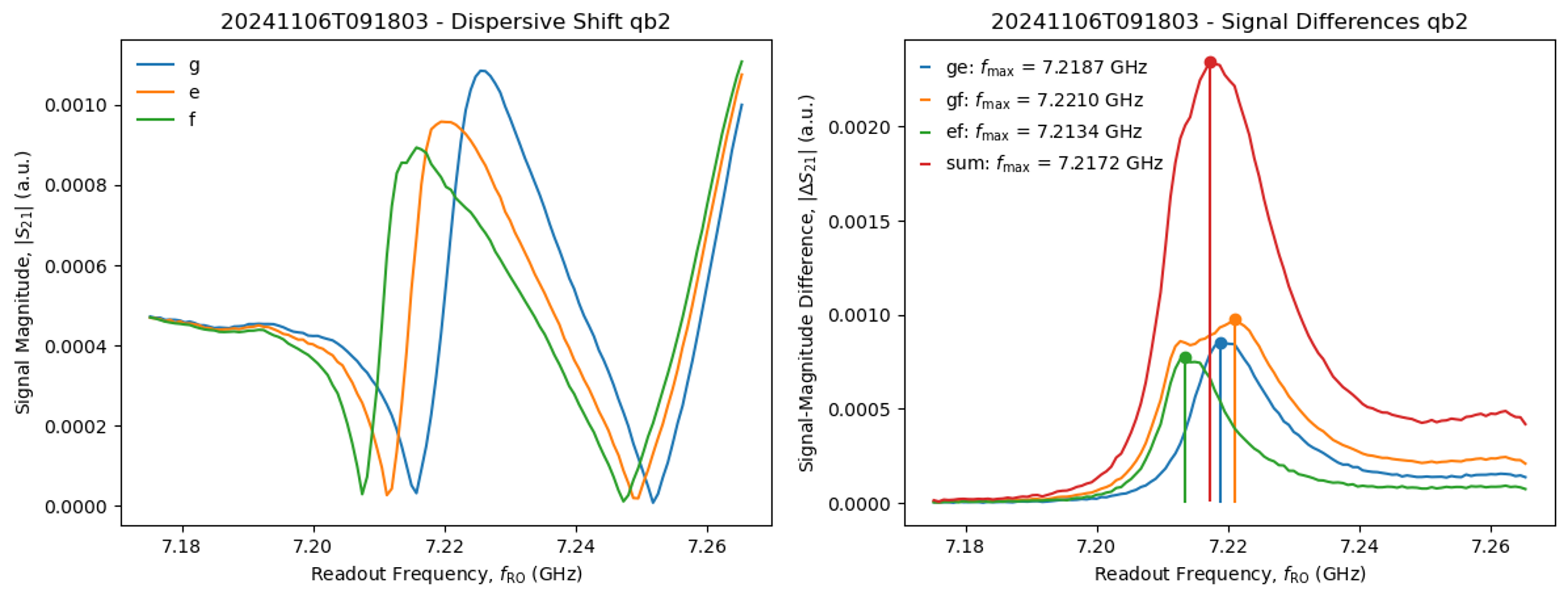
The optimal readout frequency is that at which we get the best discrimination between the qubit states. This is given by the frequency at which we get the maximum separation between the resonator lineshapes obtained when the qubit is prepared in different states. In the plot on the left, this occurs at around 7.223 GHz, where the vertical separation between the three lines is maximal (as shown by the red line in the plot on the right).
options = dispersive_shift.experiment_workflow.options()
options
qubit_to_measure = qubits[0]

options = dispersive_shift.experiment_workflow.options()
# options.close_figures(False)  # uncomment to display the analysis figures in the kernels
options.update(True)

exp_workflow = dispersive_shift.experiment_workflow(
    session=session,
    qpu=qpu,
    qubit=qubit_to_measure,
    frequencies=qubit_to_measure.parameters.readout_resonator_frequency
    + np.linspace(-50e6, 50e6, 121),
    states="gef",
    options=options,
)
workflow_result = exp_workflow.run()
IQ-Blobs Measurement
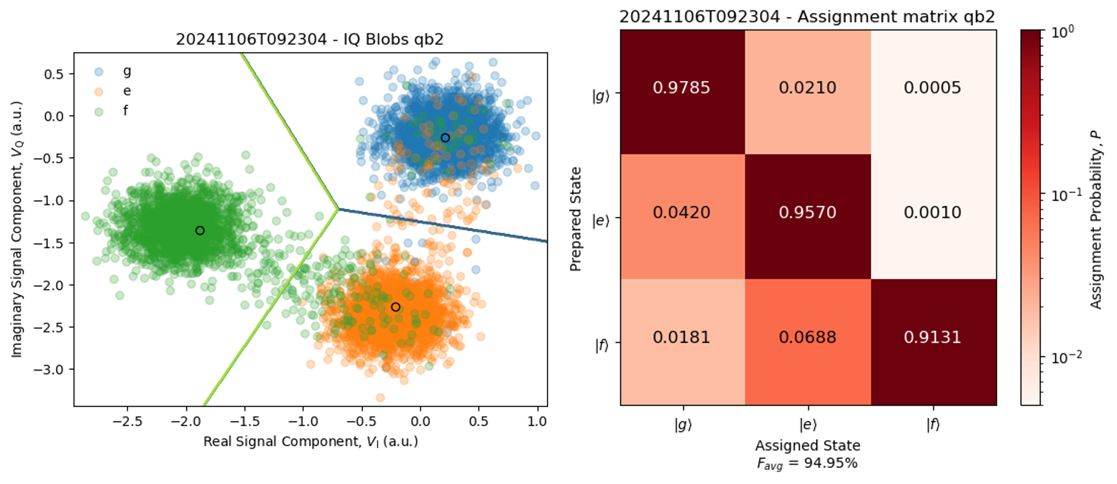
Estimate the readout fidelity from the correct state assignment probability matrix by doing a single-shot-readout measurement. Prepare the qubit in g, e, f and acquire using AveragingMode.SINGLE_SHOT.
The automated analysis calculates the assignment probability matrix and estimates the readout fidelity (also referred to here as the average assignment fidelity, $F_{avg}$.
Expect a result like this:
qubit_to_measure = qubits[0]

options = iq_blobs.experiment_workflow.options()
# options.close_figures(False)  # uncomment to display the analysis figures in the kernels
options.count(2**12)

exp_workflow = iq_blobs.experiment_workflow(
    session=session, qpu=qpu, qubits=qubit_to_measure, states="gef", options=options
)
workflow_result = exp_workflow.run()
As mentioned above, aim to obtain an average correct assignment fidelity ($F_{avg}$) greater than 90% before moving on with the tune-up of active reset. This fidelity depends on both the readout pulse amplitude and length. Find the optimal values of these parameters that give the higher readout fidelity.
Optimal Weights
Next, we want to find the integration weights that results in the best discrimination between the basis states of the qubit, and which allow us to perform multi-state discrimination.
As shown in the figure at the top of this notebook, the first processing stage in the active-reset process is a weighted integration of the acquired signal with the complex weights $w$ (often referred to as integration kernels). In the simplest case, we can set the integration weights to the real and imaginary components of a square pulse with a fixed length (maximum $2\mu$s for the QA) modulated at the readout IF frequency chosen as $f_{IF}=f_{RO}-f_{LO}$. Here, $f_{RO}$ is the readout frequency of the qubit, and $f_{LO}$ is the readout LO frequency for that qubit.
By default, each qubit has this simple integration kernel, is constructed as a constant pulse using the pulse functional pulse_library.const with amplitude = 1, and the length given by the qubit parameter:
qubits[0].parameters.readout_integration_length
This constant pulse is then modulated at the chosen IF frequency, which is stored in the qubit parameter:
qubits[
    0
].parameters.readout_frequency  # = qubits[0].parameters.readout_resonator_frequency - qubits[0].parameters.readout_lo_frequency
This modulation is done in software in order to allow multiplexed acquisition on the same QA unit, and is enabled inside the qubit calibration by setting ModulationType.SOFTWARE to the acquire-line oscillator (added automatically upon creation of the qubit):
cal[f"acquire_{qubit.uid}"] = SignalCalibration(
    oscillator = Oscillator(
        uid=f"{qubit.uid}_acquire_osc",
        frequency=self.parameters.readout_frequency,
        modulation_type=ModulationType.SOFTWARE,
    )
)
Since the readout pulse used to probe the qubit is also modulated at $f_{IF}$, the weighted integration step implements a demodulation of the acquired signal to DC. However, this demodulation process is not necessarily optimal for obtaining the best distinguishability between the readout signals for different qubit states. The so-called optimal weights which achieve this maximal distinguishability can be calculated from the measured time-traces $r_{s_i}$ of the qubit response when the qubit is prepared in the basis states that will be used for discrimination.
We measure these time traces by preparing the qubit in g, e, f and acquiring the signal response in time using AcquisitionType.RAW. Expect a result like this:

The last panel in the image above shows the extracted integration weights. The integration weights are calculated as $w_{i,j}=\overline{r_{s_i}=r_{s_j}}$, with $i, j \in {0, 1, 2, ..., n-1}$ denoting the $n$ qudit states, and $j>i$. The horizontal line denotes complex conjugation. In total, $N_w = n(n-1)/2$ integration weights are needed for distinguishing between $n$ qudit states. For example, for the qutrit case with $n=3$, we obtain the three weights $w_{0,1}=\overline{r_{s_0} - r_{s_1}}$, $w_{0,2}=\overline{r_{s_0} - r_{s_2}}$, and $w_{1,2}=\overline{r_{s_1} - r_{s_2}}$, with $r_{s_0}, r_{s_1}, r_{s_2}$ denoting the time-traces for the qutrit states g (0), e (1), f (2); see the top two panels of the image above, where we show the real and imaginary components of the measured time-traces for the states g, e, f. We've used $2^{18}$ averages, a readout-pulse length of $800$ ns and an integration length of $1~\mu$s.
Notice that $w_{1,2}=w_{0,2}-w_{0,1}$. Hence, only $w_0,1$ and $w_{0,2}$ need to be obtained from a measurement, and the remaining integration weight $w_{1,2}$ can be calculated. In general, only $n-1$ of the total of $N_w$ integration weights need to be measured, and the rest can be calculated from the pairwise differences of these measured weights. This feature is used by our instruments to enable efficient multi-state discrimination. The bottom panel in the figure above shows the two integration weights needed for discriminating a qutrit, $w_1=w_{0,1}$ and $w_2=w_{0,2}$.
The time-traces experiment workflow provided by the Applications Library measures the time traces and calculates both the optimal integration kernels $w_1,~w_2$ and the discrimination thresholds. The latter are computed as the pairwise average between the three points in the IQ plane obtained from a weighted integration of the measured time traces with the calculated weights:
$$ v_{th,i} = \cfrac{1}{2} \bigg( \sum_k w_{i,k} \cdot r_{s_0,k} + \sum_k w_{i,k} \cdot r_{s_1,k} \bigg).$$
In the equation above, $r_{s_0}$ and $r_{s_1}$ are the measured time-traces for the qudit states $s_0,s_1 \in {g, e, f, h}$, and $w_i$ is the integration weight calculated from the time-traces $r_{s_0}$ and $r_{s_1}$. The sums are over the samples $k$ of the numerical traces and weights.
Hence, the thresholds are calculated assuming equal thermal noise for the two states , which can result in a suboptimal threshold value in the case of low signal-to-noise ratio, when the distributions of the two states have significant overlap.
For $n$ discrimination states, we obtain $N_{th} = N_w = n(n-1)/2$ threshold values: as many as the total number of integration weights $N_w$. By using several acquire lines for each qubit and the calculated thresholds, we can discriminate between the $n$ qudit states during data analysis. However, the SHFQA instrument has the capability to automatically perform this multi-state discrimination and classification for every acquired shot in real-time. Below, we summarise the explanation of this process provided in the SHFQA User’s Manual and show experimental results for the multi-state discrimination of a qutrit ($n=3$).
The multi-state discrimination functionality in the SHFQA instrument classifies a signal integrated with $n-1$ weights into $n$ qudit states using $N_{th}$ discrimination thresholds and an assignment matrix specifying how the integrated signal is to be interpreted with respect to the discrimination thresholds; for example, for a qubit ($n=2$), whether $v_{sig} < v_{th}$ corresponds to state 0 or state 1, and vice versa. The process uses $N_{IU}=n-1$ integration units of the SHFQA and $N_{th}$ thresholding units. The remaining $N_{diff}=N_{th}-N_w=(n-1)(n-2)/2$ results needed by the thresholding units are calculated from the pairwise differences of the $N_{IU}$ integrated results. Thus, for example for a qutrit ($n=3$ states), $N_{IU}=2$ integration units are used and the remaining $N_{diff}=1$ result is calculated from the difference between the two integrated results; see the figure below. Finally, the thresholded results are passed to the assignment matrix, which returns a value $b\in \{ 0, 1, 2, ...\}$, corresponding to one of the $n$ qudit states $\{ g, e, f, ...\}$.
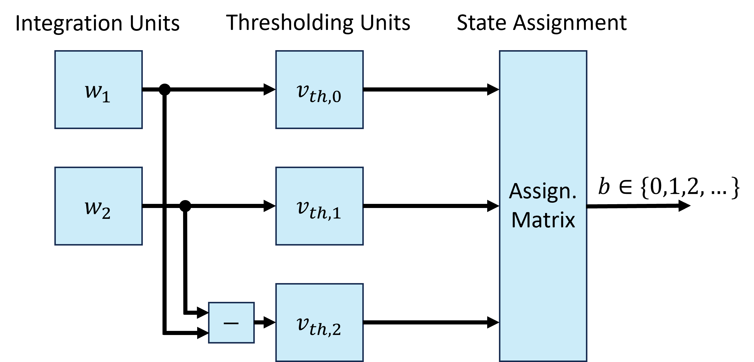
The SHFQA instrument supports discrimination of up to $n=4$ basis states; see the SHFQA User’s Manual. For $n\in \{2,3,4\}$, we give the values for $N_w$, $N_{IU}$, $N_{th}$, and in the table below.
| Number of basis states, $n$ |
Number if time traces that need to be measured, $N_{tr}=n$ |
Int. weights uploaded to QA (i. e. number of int. units needed for discrimination), $N_{UI}=n-1$ |
Total number of int. weights, $N_w=n(n-1)/2$ |
Thresholding units needed for discrimination, $N_{th}=N_w$ |
|---|---|---|---|---|
| 2 | 2 | 1 | 1 | 1 |
| 3 | 3 | 2 | 3 | 3 |
| 4 | 4 | 3 | 6 | 6 |
The optimal integration kernels and discrimination thresholds are stored in the qubit parameters readout_integration_kernels and readout_integration_discrimination_thresholds, respectively.
Running the time-traces experiment workflow with the configuration options.update(True) and options.do_analysis(True) (default) will update the two qubit parameters mentioned above with the new kernel and threshold values extracted from the analysis of the measurement. In addition, the qubit parameter readout_integration_kernels_type will be set to optimal, thus enabling the use of these optimal weights in all the weighted-integration based acquisitions of that qubit. To switch back to using the default square-shaped integration kernel, set readout_integration_kernels_type = "default".
Let's run the time-traces experiment workflow!
qubit_to_measure = qubits[0]

options = time_traces.experiment_workflow.options()
options.update(True)
# options.close_figures(False)  # uncomment to display the analysis figures in the kernels
options.count(
    2**16
)  # You typically want as many averages as you can here to have good SNR in your weights

# You can optionally choose to low-pass-filter the kernels in the analysis using the following options:
# options.filter_kernels(True)
# options.filter_cutoff_frequency(350e6)  # of the low-pass-filter
# options.granularity(16)
# options.sampling_rate(2e9)

exp_workflow = time_traces.experiment_workflow(
    session=session, qpu=qpu, qubits=qubit_to_measure, states="gef", options=options
)
workflow_result = exp_workflow.run()
Inspect the updated qubit parameters. Note that in emulation mode, the kernels are nan.
qubit_to_measure.parameters.readout_integration_kernels
qubit_to_measure.parameters.readout_integration_discrimination_thresholds
Check that readout_integration_kernels_type was set to "optimal":
qubit_to_measure.parameters.readout_integration_kernels_type
Before proceeding with the tutorial, let's manually pass some numerical values to the readout_integration_kernels so the following measurements do not fail in emulation mode.
nr_samples = len(qubit_to_measure.parameters.readout_integration_kernels[0]["samples"])
qubit_to_measure.parameters.readout_integration_kernels[0]["samples"] = np.random.rand(
    nr_samples
)
qubit_to_measure.parameters.readout_integration_kernels[1]["samples"] = np.random.rand(
    nr_samples
)
Understanding Optimal-Weights Acquisition
To understand the effect of the optimal integration weights on the data acquisition process, let's compare the result of the IQ blobs measurement performed with the standard square-shaped weights and with the optimal weights. We start with the reference measurement, using the standard square-shaped weights; see the I-Q signal plane in the first panel of the figure below. Note that this is the same measurement that was described in section IQ-Blobs Measurement, but the data was obtained during a different cooldown cycle.
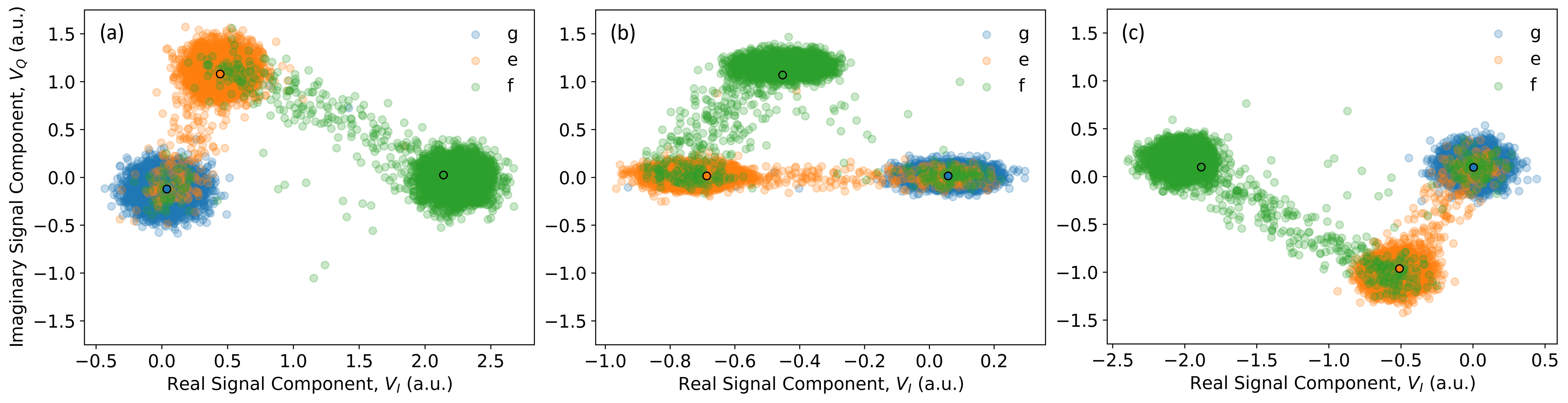
We repeat the IQ-blobs measurement using the optimal weights $w_1$. To do this, we temporarily set the qubit integration kernels to the first in the list:
qubit_to_measure = qubits[0]

options = iq_blobs.experiment_workflow.options()
# options.close_figures(False)  # uncomment to display the analysis figures in the kernels
options.count(2**12)

# get the weights
temp_pars = deepcopy(qubit_to_measure.parameters)
temp_pars.readout_integration_kernels = [
    qubit_to_measure.parameters.readout_integration_kernels[0]
]
# set the threshold corresponding to the first integration kernel
temp_pars.readout_integration_discrimination_thresholds = [
    qubit_to_measure.parameters.readout_integration_discrimination_thresholds[0]
]

exp_workflow = iq_blobs.experiment_workflow(
    session=session,
    qpu=qpu,
    qubits=qubit_to_measure,
    temporary_parameters={qubit_to_measure.uid: temp_pars},
    states="gef",
    options=options,
)
workflow_result = exp_workflow.run()
If you run the measurement above, you should find that the distributions of points for the three qutrit states are rotated such that the distributions for the states g (blue) and e (orange) lie along the horizontal, real-signal axis. We show this in the middle panel of the figure above.
Similarly, we can re-run the measurement using the weights $w_2$ by changing the index 0 to 1 in the code cell above. The result is that now the distributions for the states g (blue) and f (green) lie along the horizontal axis. We show this in the right-most panel in the figure above.
In summary, the weights $w_{i,j}$ calculated from the qudit states $i,j$ ensure that a line drawn between the distribution of integrated signals for those states is parallel to the horizontal axis (as a result of conjugation), and that these distributions are maximally separated along this axis, resulting in the best distinguishability between the states $i,j$.
Enabling Multi-State Discrimination
To enable an acquisition process that uses multi-state discrimination in LabOne Q, you simply need to pass the list of thresholds to the threshold parameter of the SignalCalibration of the acquire line, and use AcquisitionType.DISCRIMINATION in the real-time acquire loop.
If you are using the Applications Library with TunableTransmonQubit objects like the ones we have in this notebook, then you only need to set the threshold values to the qubit parameter readout_integration_discrimination_thresholds. Doing this automatically ensures that the threshold value end up in the correct SignalCalibration property.
Moreover, in the Applications Library the AcquisitionType.DISCRIMINATION mode can be easily enabled via the options in any experiment Workflow. We show this below for the IQ-blobs measurement:
qubit_to_measure = qubits[0]

options = iq_blobs.experiment_workflow.options()
# options.close_figures(False)  # uncomment to display the analysis figures in the kernels
options.count(2**12)

# Enable the discrimination mode
options.acquisition_type(AcquisitionType.DISCRIMINATION)
# Analysis is not yet implemented for the discrimination mode
# so we disabled the analysis routine here
options.do_analysis(False)

exp_workflow = iq_blobs.experiment_workflow(
    session=session, qpu=qpu, qubits=qubit_to_measure, states="gef", options=options
)
workflow_result = exp_workflow.run()
With the optimal weights used to acquire the data shown in the section Understanding Optimal-Weights Acquisition, we obtain the following result when measuring the IQ-blobs with multi-state discrimination:

We observe a state population of $p_g=0.01$ when preparing the ground state $|g\rangle$, a population of $p_e=0.96$ when preparing the excited state $|e\rangle$, and a population of $p_f=1.94$ when preparing the second-excited state $|f\rangle$, resulting in an average correct-assignment fidelity of $96.6\%$ for the discrimination process. Note that in the ideal case, $p_f=2$ because the $|f\rangle$,-state is classified as the integer $2$; see the table in section Active Reset below. The fidelity of the discrimination process is limited by thermal population and energy relaxation.
Active Reset
Refer back to the figure we have shown in the Background section. During active reset, the results of the multi-state discrimination process (the classified shot $b\in\{0,1,2,...\}$) is passed back to the signal generator. The latter can be either the SG unit of an SHFQC instrument, an SHFSG instrument, or an HDAWG instrument. A reset pulse is then played back depending on the value of $b$ as follows:
| Basis state, $s$ | Classified into, $b$ | Transitions to reset |
| :-: | :-: | :-: |
| $|g\rangle$ | 0 | No reset needed.
Qutrit is in the ground state.|
| $|e\rangle$ | 0 | $|e\rangle \rightarrow |g\rangle$ |
| $|f\rangle$ | 0 | $|f\rangle \rightarrow |e\rangle \rightarrow |g\rangle$ |
In the Applications Library, we provide a multi-qubit active_reset quantum operation, which can be used in any Experiment. Currently, you can find it in the TunableTransmonOperations. It implements active reset on qubits or qutrits.
Let's have a look at its source code to see how active reset is implemented in LabOne Q.
from laboneq_applications.qpu_types.tunable_transmon import TunableTransmonOperations

qops = TunableTransmonOperations()
qops.active_reset.src
In a similar way, you can inspect the source code of any of the other operations used inside the active_reset operation to better understand the code.
There is one subtlety about this implementation that is worth drawing attention to. As shown in the table above, resetting the qubit from the "f" state to the "g" state would ideally require two $\pi$-pulses, first on the "ef" transition, and then on the "ge" transition. Because these pulses are modulated at different IF frequencies but are played back from the same physical output of the SG instrument, a fast oscillator switch is required between these two $\pi$-pulses. However, this is not possible in a Case section. Hence, we cannot simply write:
with dsl.case():
    qops.x180(transition="ef")
    qops.x180(transition="ge")
What we must do instead to avoid an oscillator switch, is to use a special "ef" $\pi$-pulse which is software-modulated at the difference between the IF frequency of the "ef" transition and that of the "ge" transition. Then, the same instrument oscillator can be used for both pulses.
In the TunableTransmonOperations this special operation is called x180_ef_reset. Let's inspect its source code:
qops.x180_ef_reset.src
Notice reset_pulse modulated at the difference between the IF frequencies of the "ge" and "ef" transitions.
Notice also how the pulse is played on the qubit logical signal used for the "ge" drive, not the "ef" drive. This ensures that the same oscillator is used for both pulses. To learn more about the qubit method .transition_parameters, check out the tutorial on qubit and quantum operations.
The active_reset operation is integrated into all of the pulse-based experiment Workflows in the Applications Library. You can enable it via the options. Below, we show how to do this for an amplitude-Rabi experiment.
You can also easily enable a threshold-discrimination-based acquisition by setting options.acquisition_type(AcquisitionType.DISCRIMINATION).
Note: AcquisitionType.DISCRIMINATION is not needed to enable active reset. The active reset protocol is enabled by setting the qubit parameter readout_integration_discrimination_thresholds and adding the Match-Case sections to the Experiment pulse sequence.
Note: If you are using active reset, it makes sense to reduce the reset_delay_length to a few microseconds.
Below, we show how to run an amplitude-Rabi experiment workflow with active reset on the qubit states "g" and "e". The fidelity of the active reset protocol is typically limited by qubit decay and the error of the state-discrimination process. Repeating the active reset protocol a few times increases the overall reset fidelity. Below, we apply 4 repetitions.
options = amplitude_rabi.experiment_workflow.options()
# options.close_figures(False)  # uncomment to display the analysis figures in the kernels
options.count(2**12)
# Enable and configure active reset
options.active_reset(True)
options.active_reset_repetitions(4)
options.active_reset_states("ge")


qubit_to_measure = qubits[0]

# Here we change the reset_delay_length only for this experiment.
# If you continue to use active reset for all experiments, it might make sense to change the qubit parameter globally:
# qubit.parameter.reset_delay_length = 1e-6
temp_pars = deepcopy(qubit_to_measure.parameters)
temp_pars.reset_delay_length = 1e-6


workflow_result = amplitude_rabi.experiment_workflow(
    session=session,
    qpu=qpu,
    qubits=qubit_to_measure,
    temporary_parameters={qubit_to_measure.uid: temp_pars},
    amplitudes=np.linspace(0, 1, 21),
    options=options,
).run()
With the optimal weights used to acquire the data shown in the section Understanding Optimal-Weights Acquisition, we have obtained the following results when measuring the amplitude-Rabi experiment with up to 4 active reset repetitions:
