Qubit Spectroscopy
Prerequisites
This guide assumes you have a configured DeviceSetup as well as Qubit objects with assigned parameters. Please see our tutorials if you need to create your setup and qubits for the first time.
You can run this notebook on real hardware in the lab. However, if you don't have the hardware at your disposal, you can also run the notebook "as is" using an emulated session (see below).
If you are just getting started with the LabOne Q Applications Library, please don't hesitate to reach out to us at info@zhinst.com.
Background
In this how-to guide, you'll perform a measurement to determine the qubit transition frequency. The LabOne Q Applications Library provides different experiment workflows to achieve this task. You can either just sweep the frequency of a qubit drive pulse using the qubit_spectroscopy experiment workflow, or perform a 2D sweep to optimize at the same time the amplitude of the qubit drive pulse (the qubit_spectroscopy_amplitude experiment workflow).
Below is a simple diagram of showing the ground and the first excited state of a qubit, where the transition frequency corresponds to the $\omega_{01}$.

As the swept qubit drive frequency comes close to the qubit transition frequency, the qubit will be driven out of its ground state. Due to dispersive coupling (see dispersive readout how-to for more detail), the signal from the readout resonator will then experience a shift in magnitude and phase.
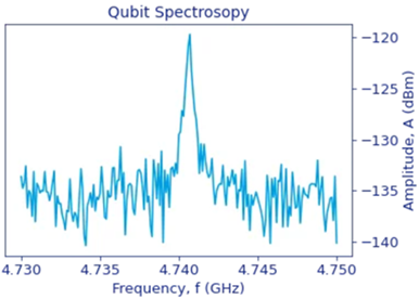
Plotting the readout signal, we can obtain a lorentzian lineshape as a function of the qubit drive frequency. This lorentzian will be centered around the qubit transition frequency, and from its linewidth we can approximate the qubit dephasing time. Below is an example dataplot of a qubit spectroscopy measurement:
Imports
You'll start by importing laboneq.simple.
from laboneq.simple import *
Define your experimental setup
Let's define our experimental setup. We will need:
a set of TunableTransmonOperations
a QPU
Here, we will be brief. We will mainly provide the code to obtain these objects. To learn more, check out these other tutorials:
We will use 3 TunableTransmonQubits in this guide. Change this number to the one describing your setup.
number_of_qubits = 3
DeviceSetup
This guide requires a setup that can drive and readout tunable transmon qubits. Your setup could contain an SHFQC+ instrument, or an SHFSG and an SHFQA instruments. Here, we will use an SHFQC+ with 6 signal generation channels and a PQSC.
If you have used LabOne Q before and already have a DeviceSetup for your setup, you can reuse that.
If you do not have a DeviceSetup, you can create one using the code below. Just change the device numbers to the ones in your rack and adjust any other input parameters as needed.
# Setting get_zsync=True below, automatically detects the zsync ports of the PQCS that
# are used by the other instruments in this descriptor.
# Here, we are not connected to instruments, so we set this flag to False.
from laboneq.contrib.example_helpers.generate_descriptor import generate_descriptor

descriptor = generate_descriptor(
    pqsc=["DEV10001"],
    shfqc_6=["DEV12001"],
    number_data_qubits=number_of_qubits,
    multiplex=True,
    number_multiplex=number_of_qubits,
    include_cr_lines=False,
    get_zsync=False,  # set to True when at a real setup
    ip_address="localhost",
)
setup = DeviceSetup.from_descriptor(descriptor, "localhost")
Qubits
We will generate 3 TunableTransmonQubits from the logical signal groups in our DeviceSetup. The names of the logical signal groups, q0, q1, q2, will be the UIDs of the qubits. Moreover, the qubits will have the same logical signal lines as the ones of the logical signal groups in the DeviceSetup.
from laboneq_applications.qpu_types.tunable_transmon import TunableTransmonQubit

qubits = TunableTransmonQubit.from_device_setup(setup)
for q in qubits:
    print("-------------")
    print("Qubit UID:", q.uid)
    print("Qubit logical signals:")
    for sig, lsg in q.signals.items():
        print(f"  {sig:<10} ('{lsg:>10}')")
Configure the qubit parameters to reflect the properties of the qubits on your QPU using the following code:
for q in qubits:
    q.parameters.ge_drive_pulse["sigma"] = 0.25
    q.parameters.readout_amplitude = 0.5
    q.parameters.reset_delay_length = 1e-6
    q.parameters.readout_range_out = -25
    q.parameters.readout_lo_frequency = 7.4e9

qubits[0].parameters.drive_lo_frequency = 6.4e9
qubits[0].parameters.resonance_frequency_ge = 6.3e9
qubits[0].parameters.resonance_frequency_ef = 6.0e9
qubits[0].parameters.readout_resonator_frequency = 7.0e9

qubits[1].parameters.drive_lo_frequency = 6.4e9
qubits[1].parameters.resonance_frequency_ge = 6.5e9
qubits[1].parameters.resonance_frequency_ef = 6.3e9
qubits[1].parameters.readout_resonator_frequency = 7.3e9

qubits[2].parameters.drive_lo_frequency = 6.0e9
qubits[2].parameters.resonance_frequency_ge = 5.8e9
qubits[2].parameters.resonance_frequency_ef = 5.6e9
qubits[2].parameters.readout_resonator_frequency = 7.2e9
Quantum Operations
Create the set of TunableTransmonOperations:
from laboneq_applications.qpu_types.tunable_transmon import TunableTransmonOperations

qops = TunableTransmonOperations()
QPU
Create the QPU object from the qubits and the quantum operations
from laboneq.dsl.quantum import QPU

qpu = QPU(qubits, quantum_operations=qops)
Alternatively, load from a file
If you you already have a DeviceSetup and a QPU stored in .json files, you can simply load them back using the code below:
from laboneq import serializers

setup = serializers.load(full_path_to_device_setup_file)
qpu = serializers.load(full_path_to_qpu_file)

qubits = qpu.quantum_elements
qops = qpu.quantum_operations
Connect to Session
session = Session(setup)
session.connect(do_emulation=True)  # do_emulation=False when at a real setup
Create a FolderStore for Saving Data
The experiment Workflows can automatically save the inputs and outputs of all their tasks to the folder path we specify when instantiating the FolderStore. Here, we choose the current working directory.
# import FolderStore from the `workflow` namespace of LabOne Q, which was imported
# from `laboneq.simple`
from pathlib import Path

folder_store = workflow.logbook.FolderStore(Path.cwd())
We disable saving in this guide. To enable it, simply run folder_store.activate().
folder_store.deactivate()
Optional: Configure the LoggingStore
You can also activate/deactivate the LoggingStore, which is used for displaying the Workflow logging information in the notebook; see again the tutorial on Recording Experiment Workflow Results for details.
Displaying the Workflow logging information is activated by default, but here we deactivate it to shorten the outputs, which are not very meaningful in emulation mode.
We recommend that you do not deactivate the Workflow logging in practice.
from laboneq.workflow.logbook import LoggingStore

logging_store = LoggingStore()
logging_store.deactivate()
Running the Experiment Workflow
You'll now instantiate the experiment workflow and run it. For more details on what experiment workflows are and what tasks they execute, see the Experiment Workflows tutorial.
You'll start by importing numpy, the qubit-spectroscopy experiment workflows from laboneq_applications, as well as plot_simulation for inspecting the experiment sequence.
import numpy as np
from laboneq.contrib.example_helpers.plotting.plot_helpers import plot_simulation

from laboneq_applications.experiments import (
    qubit_spectroscopy,
    qubit_spectroscopy_amplitude,
)
Let's first create the options class for the qubit-spectroscopy experiment and inspect it using the show_fields function from the workflow namespace of LabOne Q, which was imported from laboneq.simple:
options = qubit_spectroscopy.experiment_workflow.options()
workflow.show_fields(options)
Notice that, unless we change it:
- the experiment is run in
AcquisitionType.INTEGRATIONandAveragingMode.CYCLIC, using 1024 averages (count) - there is a waiting time of 1$\mu$s between the end of every acquisition and the playback of the subsequent readout pulse (
spectroscopy_reset_delay) - the analysis workflow will run automatically (
do_analysis=True) - the figures produced by the analysis are automatically closed (
close_figures=True) - the qubit parameters will not be updated (
update=False)
Here, let's disable closing the figures produced by the analysis so we see them in the cell output. Note however that the fit attempted by the analysis routine in emulation mode will not be representative, because we do not acquire data from a real experiment.
options.close_figures(False)
Now we run the experiment workflow on the first two qubits in parallel.
# our qubits live here in the demo setup:
qubits = qpu.quantum_elements

exp_workflow = qubit_spectroscopy.experiment_workflow(
    session=session,
    qpu=qpu,
    qubits=[qubits[0].uid, qubits[1].uid],
    frequencies=[np.linspace(5.8e9, 6.2e9, 101), np.linspace(5.9e9, 6.3e9, 101)],
    options=options,
)

workflow_results = exp_workflow.run()
Inspect the Tasks That Were Run
for t in workflow_results.tasks:
    print(t)
Inspect the Output Simulation
You can also inspect the compiled experiment and plot the simulated output:
compiled_experiment = workflow_results.tasks["compile_experiment"].output
plot_simulation(compiled_experiment, length=50e-6, signal_names_to_show=["measure"])
Inspecting the Source Code of the Pulse-Sequence Creation Task
You can inspect the source code of the create_experiment task defined in ramsey to see how the experiment pulse sequence is created using quantum operations. To learn more about the latter, see the Quantum Operations tutorial.
qubit_spectroscopy.create_experiment.src
To learn more about how to work with experiment Workflows, check out the Experiment Workflows tutorial.
Here, let's briefly inspect the analysis-workflow results.
Analysis Results
Let's check what tasks were run as part of the analysis workflow:
analysis_workflow_results = workflow_results.tasks["analysis_workflow"]
for t in analysis_workflow_results.tasks:
    print(t)
We can access the qubit parameters extracted by the analysis from the output of the analysis-workflow:
from pprint import pprint

pprint(analysis_workflow_results.output)
Check out the Experiment Workflows tutorial to see how you can manually update the qubit parameters to these new values, or reset them to the old ones.
Sweep the amplitude at the same time
Getting back to our found parameters, we now repeat the workflow while sweeping the amplitude of the drive frequency at the same time. Since the analysis and the interface are different, a dedicated workflow is used, but the input only differs slightly.
Since the amplitude is swept in the outer loop, while frequency is swpet in the inner loop, we set the frequency sweep to only 2 to have the amplitude modification visible in the OutputSimulator.
exp_workflow_amp = qubit_spectroscopy_amplitude.experiment_workflow(
    session=session,
    qpu=qpu,
    qubits=[qubits[0].uid, qubits[1].uid],
    amplitudes=[np.linspace(0.1, 0.5, 2), np.linspace(0.1, 0.5, 2)],
    frequencies=[np.linspace(5.8e9, 6.2e9, 3), np.linspace(5.9e9, 6.3e9, 3)],
)

workflow_results_amp = exp_workflow_amp.run()
compiled_experiment_amp = workflow_results_amp.tasks["compile_experiment"].output
plot_simulation(compiled_experiment_amp, length=50e-6)
Great! You've now run your qubit-spectroscopy experiment. Check out other experiments in this manual to keep characterizing your qubits.