Triggering and Synchronization
Note
This tutorial is applicable to all SHFQC+ Instruments.
Goals and Requirements
The goal of this tutorial is to show how to use the Signal Generator channels of the SHFQC+ as a trigger source, as well as how to configure the SHFQC+ to respond to an external trigger. In order to visualize the multi-channel signals, an oscilloscope with sufficient bandwidth and channel number is required. This can be an external scope, or the scope of the SHFQC+, for which a loopback configuration is needed with the Quantum Analyzer channel.
Preparation
Connect the cables as illustrated below. Make sure that the instrument is powered on and connected by Ethernet to your local area network (LAN) where the host computer resides. After starting LabOne, the default web browser opens with the LabOne graphical user interface.
Note
The instrument can also be connected via the USB interface, which can be simpler for a first test. As a final configuration for measurements, it is recommended to use the 1GbE interface, as it offers a larger data transfer bandwidth.

The tutorial can be started with the default instrument configuration (e.g. after a power cycle) and the default user interface settings (e.g. after pressing F5 in the browser).
Generating and Responding to Triggers
In this tutorial you will learn about the most important use cases:
- Generating a TTL signal with the AWG to trigger another piece of equipment
- Triggering the Signal Generator channels of the AWG with an external TTL signal
Generating Markers with the AWG
To begin with, we generate a trigger output with the Signal Generator channel 1. As this tutorial is an extension of the Basic Waveform Playback Tutorial, configure the SHFQC+ as follows:
| Tab | Sub-tab | Label | Setting / Value / State |
|---|---|---|---|
| In/Out | SG Channel 1 | On | ON |
| In/Out | SG Channel 1 | Range (dBm) | 10 |
| In/Out | SG Channel 1 | Center Freq (Hz) | 1.0 G |
| In/Out | SG Channel 1 | Output Path | RF |
| In/Out | SG Channel 2 | On | ON |
| In/Out | SG Channel 2 | Range (dBm) | 10 |
| In/Out | SG Channel 2 | Center Freq (Hz) | 1.0 G |
| In/Out | SG Channel 2 | Output Path | RF |
| Scope Setting | Value / State |
|---|---|
| Ch1 enable | ON |
| Ch1 range | 0.2 V/div |
| Ch2 enable | ON |
| Ch2 range | 0.5 V/div |
| Timebase | 500 ns/div |
| Trigger source | Ch2 |
| Trigger level | 200 mV |
| Run / Stop | ON |
After configuring the output using the table above, we use the SHFQC+ to generate a trigger output. There are two ways of generating trigger output signals with the Signal Generators AWG: as markers that are part of a waveform and played with sample precision, or by controlling trigger bits through the sequencer.
The method using markers is recommended when precise timing is required, and/or complicated serial bit patterns need to be played on the Marker outputs. Marker bits are part of every waveform, and are set to zero by default. Each waveform is represented by an array of 16-bit words: 14 bits of each word represent the analog waveform data, and the remaining 2 bits represent two digital marker channels. Hence, upon playback, a digital signal with sample-precise alignment with the analog output is generated.
Generating a TTL output signal using a sequencer instruction is simpler, but the timing resolution is lower than when using markers. The sequencer instructions play at the sequencer clock cycle of 4 ns, whereas the markers are part of the waveform and therefore have a resolution of 0.5 ns. The method using sequencer instructions is useful to generate a single trigger signal at the start of an AWG program, for instance.
| Marker | Trigger | |
|---|---|---|
| Implementation | Part of waveform | Sequencer instruction |
| Timing control | High | Low |
| Generation of serial bit patterns | Yes | No |
| Cross-device synchronization | Yes | Yes |
Let us first demonstrate the use of markers. In the following code
example we first generate a Gaussian pulse. This is identical as in the
Basic Waveform Playback Tutorial, where the
generated wave already included marker bits - they were simply set to
zero by default. We use the marker function to assign the desired
non-zero marker bits to the wave. The marker function takes two
arguments: the first is the length of the wave in samples; the second is
the marker configuration in binary encoding, where the value 0 stands
for both marker bits low, the values 1, 2, and 3 stand for the first,
the second, and both marker bits high, respectively. We use this to
construct the wave called w_marker.
const marker_pos = 3000;

wave w_gauss  = gauss(8000, 4000, 1000);
wave w_left   = marker(marker_pos, 0);
wave w_right  = marker(8000-marker_pos, 1);
wave w_marker = join(w_left, w_right);
wave w_gauss_marker = w_gauss + w_marker;

playWave(1, w_gauss_marker);
The waveform addition with the '+' operator adds up analog waveform data
but also combines marker data. The wave w_gauss contains zero marker
data, whereas the wave w_marker contains zero analog data.
Consequently the wave called w_gauss_marker contains the merged analog
and marker data. We use the integer constant marker_pos to determine
the point where the first marker bit flips from 0 to 1 somewhere in the
middle of the Gaussian pulse.
Note
The add function and the '+' operator combine marker bits by a logical OR operation. This means combining 0 and 1 yields 1, and combining 1 and 1 yields 1 as well.
There is a certain freedom to assign different marker bits to the Mark outputs. The following table summarizes the settings to apply in order to output marker bit 1 on the Mark output of the Signal Generator channel 1. (% else -$) Mark 1.
| Tab | Sub-tab | Section | # | Label | Setting / Value / State |
|---|---|---|---|---|---|
| DIO | Marker Out | 1 | Signal | Output 1 Marker 1 |
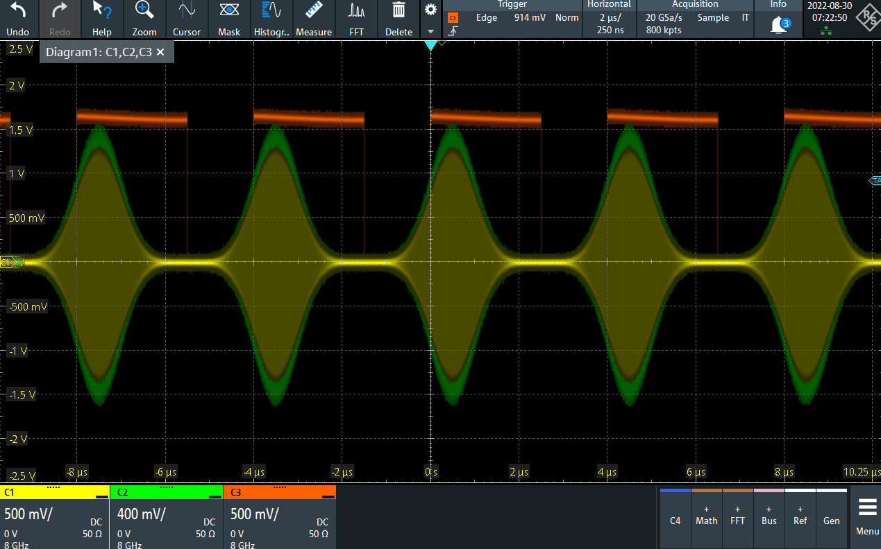
Figure 2 shows the AWG
signal captured by the scope as a yellow curve. The green curve shows
the second scope channel displaying the marker signal. Try changing the
marker_pos constant and re-running the sequence program to observe the
effect on the temporal alignment of the Gaussian pulse. After the
waveform has finished playing, the marker bit returns to a value of zero
automatically, as no more waveform is being played.
Let us now demonstrate the use of sequencer instructions to generate a trigger signal. Copy and paste the following code example into the Sequence Editor.
wave w_gauss = gauss(8000, 4000, 1000);

setTrigger(1);
playWave(1, w_gauss);
waitWave();
setTrigger(0);
Each AWG core has four trigger output states available to it. The
setTrigger function takes a single argument encoding the four trigger
output states in binary manner – the integer number 1 corresponds to a
configuration of 0/0/0/1 for the trigger outputs 4/3/2/1. The binary
integer notation of the form 0b0000 is useful for this purpose – e.g.
setTrigger(0b0011) will set trigger outputs 1 and 2 to 1, and trigger
outputs 3 and 4 to 0. We included a waitWave instruction after the
playWave instruction. It ensures that the subsequent setTrigger
instruction is executed only after the Gaussian wave has finished
playing, and not during waveform playback.
Note
The waitWave instruction represents a means to control the timing of
instructions in the Wait & Set and the Playback queues. In the example
above, the waitWave instruction puts the playback of the next
instruction in the Wait & Set queue, in this case setTrigger(0), on
hold until the waveform is finished. Without the waitWave instruction,
the AWG trigger would return to zero at the beginning of the waveform
playback.
Note
The use of waitWave is explicitly not required between consecutive
playWave and playZero instructions. Sequential instructions in the
Playback queue are played immediately after one another, back to back.
We reconfigure the Mark 1 connector in the DIO tab such that it outputs
AWG Trigger 1, instead of Output 1 Marker 1. The rest of the
settings can stay unchanged.
| Tab | Sub-tab | Section | # | Label | Setting / Value / State |
|---|---|---|---|---|---|
| DIO | Marker Out | 1 | Signal | AWG Trigger 1 |
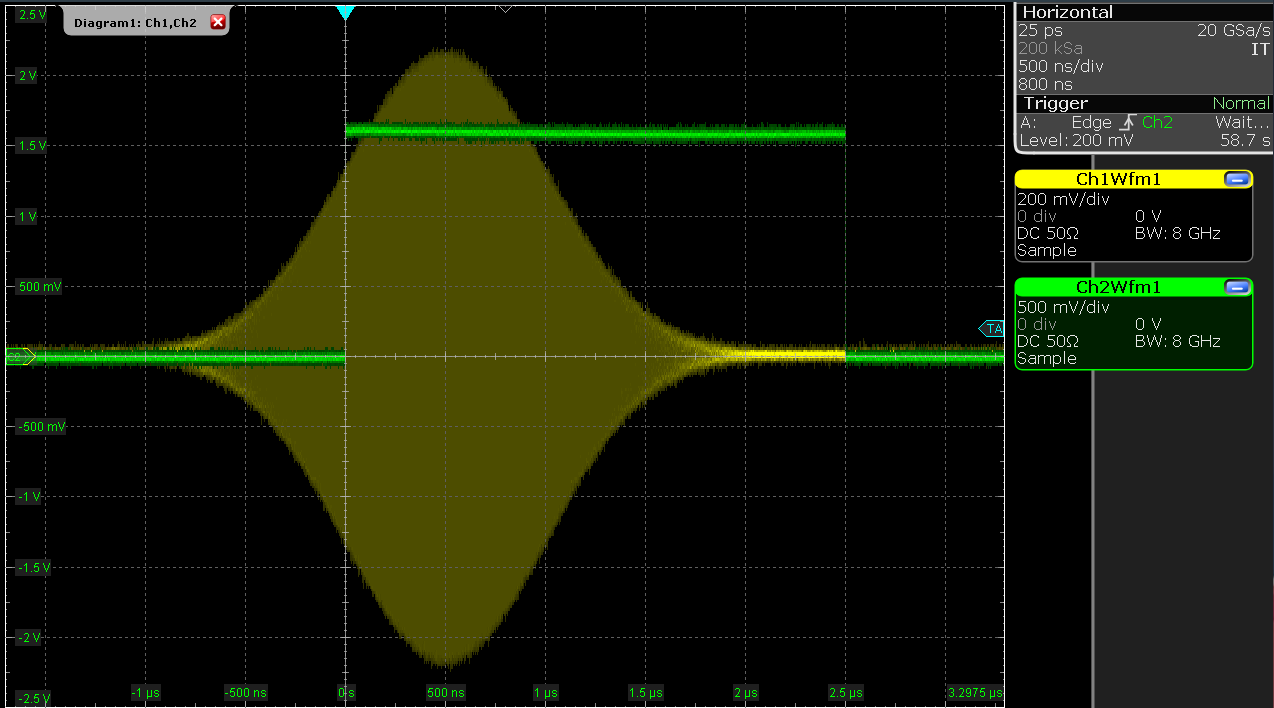
Figure 3 shows the AWG signal captured by the scope. This looks very similar to Figure 2 in fact. With this method, we’re less flexible in choosing the trigger time, as the rising trigger edge will always be at the beginning of the waveform. But we don’t have to bother about assigning the marker bits to the waveform.
Triggering the AWG
Note
This section shows how to use the SHFQC+ to generate and respond to external triggers. To synchronize the outputs of different channels on the same SHFQC+, it is recommended to use the Internal Trigger Unit.
For this part of the tutorial, connect the cables as illustrated below.

In this section we show how to trigger the AWG with an external TTL signal. We start by using the Signal Generator channel 1 of the SHFQC+ to generate a periodic TTL signal. As shown in Figure 4, the Mark output of channel 1 is connected to the Trig input of channel 2. We monitor the marker and signal outputs of channel 2 on a scope.
wave m_high = marker(8000,1); //marker high for 8000 samples
wave m_low = marker(8000,0); //marker low for 8000 samples
wave m = join(m_high, m_low);

while (1) {
    playWave(m);
}
Compile and run the above program on the AWG core of channel 1. Then
configure the Mark 1 and Mark 2 to use Output 1 Marker 1:
| Tab | Sub-tab | Section | # | Setting / Value / State |
|---|---|---|---|---|
| DIO | Marker | Source | 1 | Output 1 Marker 1 |
| DIO | Marker | Source | 2 | Output 1 Marker 1 |
Next we configure channel 2 to respond to the trigger generated by channel 1. Internally, the AWG core of each channel has 2 digital trigger input channels. These are not directly associated with physical device inputs but can be freely configured to probe a variety of internal or external signals. Here, we link the AWG Digital Trigger 1 of Channel 2 to the physical Trig 2 connector, and we configure it to trigger on the rising edge.
| Tab | # | Sub-tab | Section | Label | Setting / Value / State |
|---|---|---|---|---|---|
| AWG | 2 | Trigger | Digital Trigger 1 | Signal | Trigger In 2 |
| AWG | 2 | Trigger | Digital Trigger 1 | Slope | Rise |
Finally, we modify the previous AWG program by adding a while loop so
that the sequence can be repeated infinitely and by including a
waitDigTrigger instruction just before the playWave instruction. The
result is that upon every repetition inside the infinite while loop,
the AWG will wait for a rising edge on Trig 2.
const marker_pos = 3000;

wave w_gauss  = gauss(8000, 4000, 1000);
wave w_left   = marker(marker_pos, 0);
wave w_right  = marker(8000-marker_pos, 1);
wave w_marker = join(w_left, w_right);
wave w_gauss_marker = w_gauss + w_marker;

while (1) {
    //wait for external trigger
    waitDigTrigger(1);
    playWave(1, w_gauss_marker);
}
Compile and run the above program on the AWG core of channel 2.
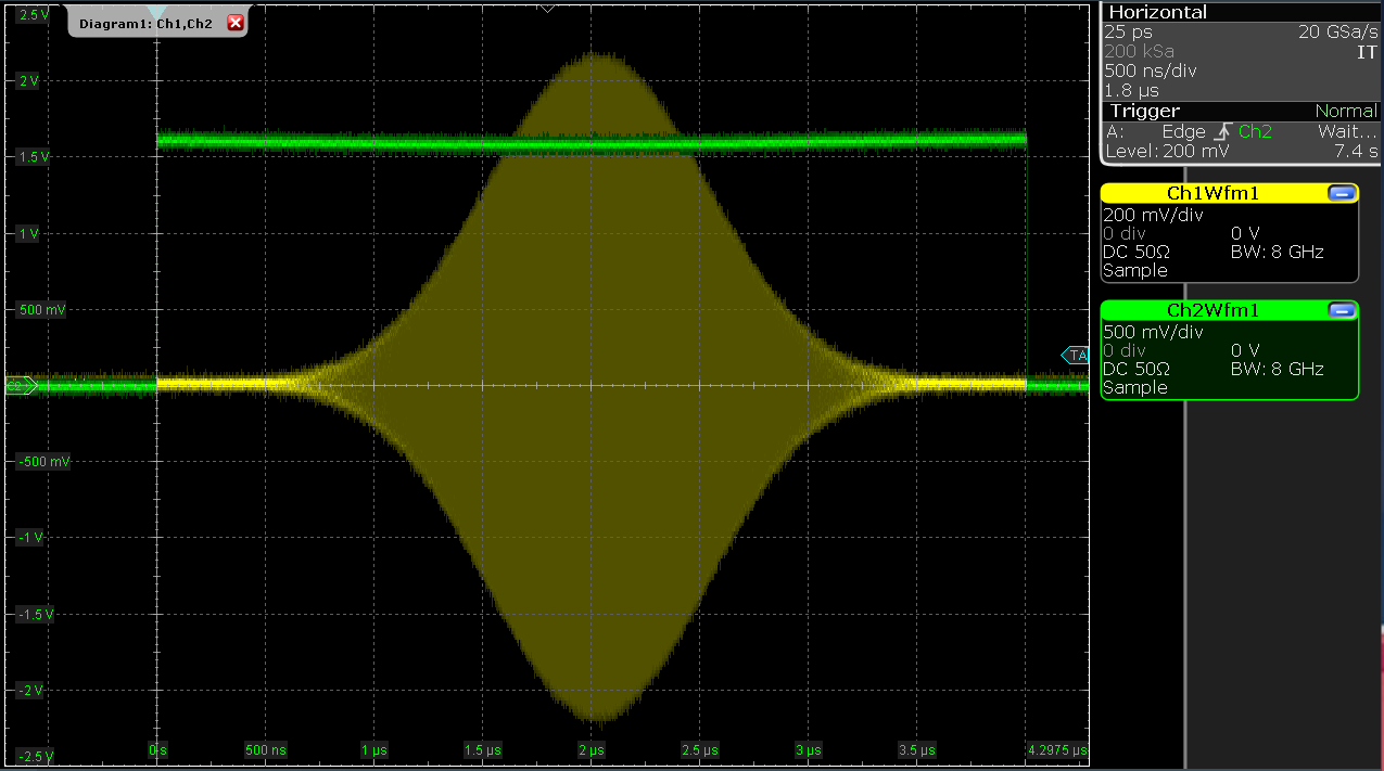
Figure 5 shows the pulse series as seen on
the scope: the pulses are now spaced by the oscillator period of 8 μs,
unlike previously when the period was determined by the length of the
waveform w_gauss. Try changing the trigger signal frequency or
unplugging the trigger cable to observe the immediate effect on the
signal.
Synchronizing outputs of different channels
For this part of the tutorial, connect the cables as illustrated below.

In this section we will show how to use the Internal Trigger Unit to synchronize the outputs of multiple channels of the SHFQC+.
Note
In this tutorial, we show how to synchronize two Signal Generator
Channel outputs of the SHFQC+, but the Internal Trigger Unit can also be
used to synchronize the Quantum Analyzer and Signal Generator channel
outputs with each other by using the waitDigTrigger command in the
Quantum Analyzer sequence and configuring the digital trigger of the
Quantum Analyzer channel to use the Internal Trigger Unit.
To configure the internal trigger, set the following settings in the tables below.
| Tab | Sub-tab | Section | # | Setting / Value / State |
|---|---|---|---|---|
| DIO | Internal Trigger | Repetitions | 1e9 | |
| DIO | Internal Trigger | Holdoff | 100 ns |
| Tab | # | Sub-tab | Section | Label | Setting / Value / State |
|---|---|---|---|---|---|
| AWG | 1 | Trigger | Digital Trigger 1 | Signal | Internal Trigger |
| AWG | 2 | Trigger | Digital Trigger 1 | Signal | Internal Trigger |
The number of repetitions (ranging from 1 to more than 1e9) determines how many triggers will be sent out. The holdoff time (minimum 100 ns, resolution of 100 ns, maximum 4000 s) determines the time in seconds between the individual trigger events, typically chosen to be longer than the longest part of the sequence. For example, in a Ramsey experiment, the hold-off time might be slightly longer than the length of two pi/2-pulses plus the length of the longest evolution time and the length of the readout pulse. After entering the settings above, the Internal Trigger Unit is configured but is not yet sending out triggers. We will enable the triggers after uploading our sequences.
Compile and run the sequencer code below (which is the same as in the section above) to SG channels 1 and 2 of the SHFQC+.
const MARKER_POS = 3000;

wave w_gauss  = gauss(8000, 4000, 1000);
wave w_left   = marker(MARKER_POS, 0);
wave w_right  = marker(8000-MARKER_POS, 1);
wave w_marker = join(w_left, w_right);
wave w_gauss_marker = w_gauss + w_marker;

while (1) {
    //wait for internal trigger
    waitDigTrigger(1);
    playWave(1,2, w_gauss_marker);
}
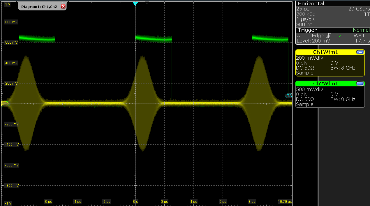
The sequencers are now waiting until they receive a trigger. Enable the
internal trigger by clicking Run/Stop button in the Internal Trigger
section of the DIO Tab. Figure 7 shows that the outputs of channels 1
and 2 are synchronized in time.