Quantum Analyzer Setup Tab¶

The Quantum Analyzer Setup is the main control panel for the qubit measurement unit on the Instrument (see Functional Overview for an overview block diagram). It is available on all SHFQC+ Instruments.

Features¶

Spectroscopy mode and readout mode
Continuous or pulsed resonator spectroscopy
Power spectral density
Weighted integration
Readout up to 16 qubits per channel
2-state and multistate discrimination

Description¶

The Quantum Analyzer Setup tab is divided into 2 sub-tab groups for resonator spectroscopy (see Figure 1) and qubit readout (see Figure 2) application. By selecting Application Mode, Spectroscopy or Readout, the corresponding sub-tabs provide all configurations of readout pulse generation and acquired data processing (see ). The main differences of the Application Modes are listed in Table 2.

Figure 1: LabOne GUI: QA Setup Tab - Spectroscopy Mode

Figure 2: LabOne GUI: QA Setup Tab - Readout Mode

Figure 3: LabOne GUI: Readout Pulse Generator Tab - Waveform Viewer

Table 2: Main differences of Spectroscopy and Readout mode
Parameters	Spectroscopy mode	Readout mode
Waveform generation	Digital oscillator and envelope	Sample by Sample
Waveform output mode	Continuous or pulsed	Pulsed
Waveform length	Continuous or up to 16 μs or 32 μs	Up to 2 μs
Number of qubits per channel	1	Up to 8 or 16
Integration length	Up to 16.7 ms	Up to 2 μs
Integration weight unit per channel	Not applicable	Up to 8 or 16
Result normalization after integration	Normalized by integration length in samples	Not normalized
Real-time state discrimination	Not applicable	Yes
Multistate discrimination	Not applicable	Qubits, qutrits and ququads

Spectroscopy Mode¶

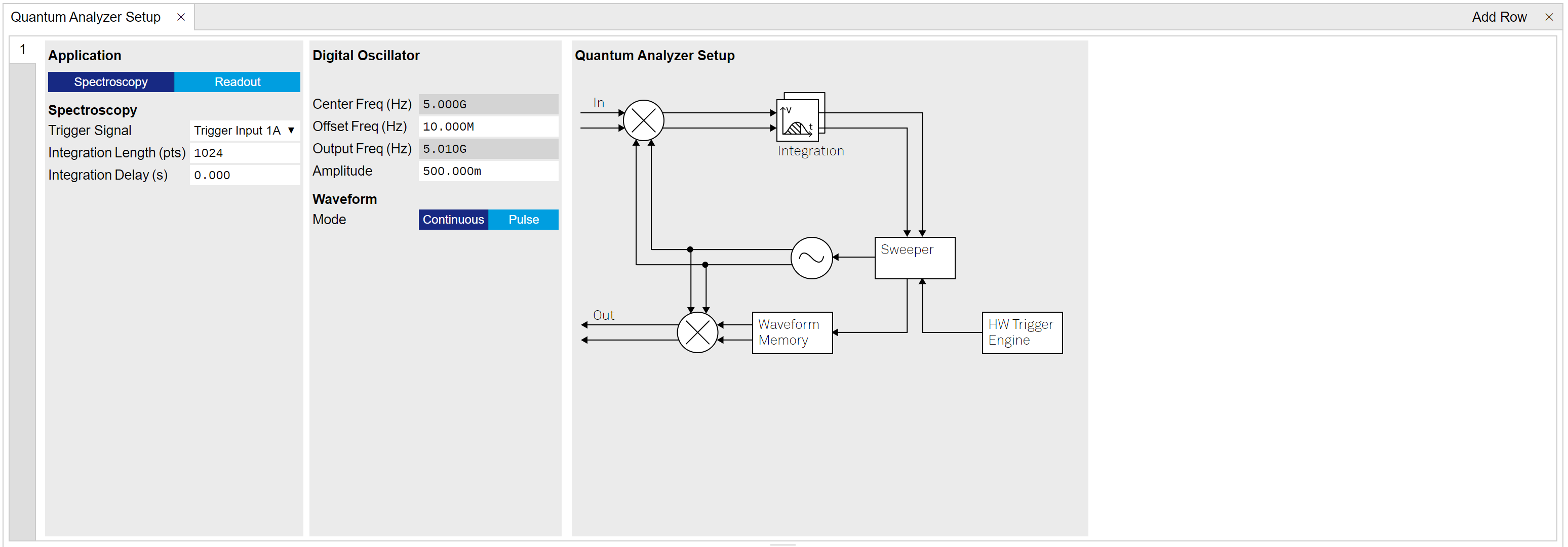
Spectroscopy mode is mainly used for resonator spectroscopy and power spectral density measurement. The SHFQC+ has 1 Digital Oscillator per Quantum Analyzer channel. In Spectroscopy mode, the Digital Oscillator is used for readout waveform generation and integration. The SHFQC+ Sweeper class (API) is the central controller for the Spectroscopy mode, see tutorial Continuous Resonator Spectroscopy and Pulsed Resonator Spectroscopy.

There are 2 operation modes for readout waveform generation, Continuous and Pulsed. In Continuous mode, signal from the Digital Oscillator is routed to the digital IQ mixing stage (see Functional Overview) for readout waveform generation in the output path, and to multiply the input signal for readout waveform integration in the input path, see Figure 4. In Pulsed mode, signal from the Digital Oscillator modulates the envelope from the Waveform Memory and then is routed to the output and input paths same as in Continuous mode. The pulse envelope can be displayed on the Waveform Viewer sub-tab of the Readout Pulse Generator tab. The main differences of the 2 operation modes are listed in Table 3.

Figure 4: Readout waveform generation and integration in Spectroscopy mode

Table 3: Main differences of Continuous and Pulsed mode in Spectroscopy
Parameters	Continuous mode	Pulsed mode
Readout pulse length	Continuous wave	Up to 16 μs or 32 μs (up to 32 kSa or 64 kSa)
Envelope delay	Not applicable	Up to 131.1 μs
Readout pules amplitude	Controlled by output range and gain factor of the Digital Oscillator	Controlled by output range, gain factor of the Digital Oscillator and the envelope

Readout Waveform Output In Spectroscopy Mode¶

The readout waveform on the Instrument output can be expressed as

\[ \begin{equation}\tag{1} E_{\mathrm{output}}(t) = C_{P\rightarrow A}\operatorname{Re}[A(t)g_{\mathrm{osc}}e^{i2\pi (f_0 + f_{\mathrm{osc}}) t + i\phi_{\mathrm{output}}}], \end{equation} \]

where \(C_{P\rightarrow A} = 10^{\frac{P_{\mathrm{range,\ output}}-10}{20}}\) is the conversion factor converting the power range \(P_{\mathrm{range,\ output}}\) of the output signal in units of dBm to the amplitude in units of V, , \(A(t)\) is the complex readout envelope in Pulsed mode and \(A(t) = 1\) in Continuous mode, \(g_{\mathrm{osc}}\) is the amplitude gain factor of the baseband Digital Oscillator. The frequency \(f_{\mathrm{osc}}\) is the offset frequency set by the baseband Digital Oscillator and \(\phi_{\mathrm{output}}\) is the global phase, which can be reset by resetting the phase of the baseband Digital Oscillator. The frequency \(f_0\) is the RF center frequency set in the Input/Output tab. Note: when using the LF path the center frequency from the Input/Output tab does not apply and one has to set \(f_0 = 0\) in the above formula.

The readout waveform envelope \(A(t)\) in Pulsed mode can be displayed on the Waveform Viewer, see Figure 3.

Readout Results In Spectroscopy Mode¶

The readout input signal after analog frequency down-conversion before the ADC is

\[ \begin{equation}\tag{2} \begin{aligned} E_{\mathrm{before\ ADC}}(t) & = \operatorname{Re}(A_{\mathrm{input}}(t)e^{i2\pi f_{\mathrm{before\ ADC}} t + i\phi_{\mathrm{input}}})\\\ & = A_{\mathrm{input}}(t)\cos({2\pi f_{\mathrm{before\ ADC}} t + \phi_{\mathrm{input}}})\\\ & = A_{\mathrm{input}}(t)\frac{e^{i2\pi f_{\mathrm{before\ ADC}} t + i\phi_{\mathrm{input}}} + e^{-i2\pi f_{\mathrm{before\ ADC}} t - i\phi_{\mathrm{input}}}}{2}, \end{aligned} \end{equation} \]

where \(A_{\mathrm{input}}(t)\) is the amplitude of input signal on the front panel of the instrument, \(f_{\mathrm{before\ ADC}}\) is the frequency of the input signal before ADC, \(\phi_{\mathrm{input}}\) is the global phase of the input signal on the front panel of the instrument. After the ADC, it becomes

\[ \begin{equation}\tag{3} E_{i,\ \mathrm{after\ ADC}} = \frac{C_{\mathrm{scaling}}A_{i,\ \mathrm{input}}}{2}(e^{i2\pi f_{\mathrm{after\ ADC}} t_i + i\phi_{\mathrm{input}}} + e^{-i2\pi f_{\mathrm{after\ ADC}} t_i - i\phi_{\mathrm{input}}}), \end{equation} \]

where \(C_{\mathrm{scaling}}\) is the conversion factor depending on gain factor, ADC range and bit resolution, \(f_{\mathrm{after\ ADC}}\) is the frequency after the ADC, \(i\) means the \(i\)-th sample. The signal \(E_{i,\ \mathrm{after\ ADC}}\) is then down-converted by a digital oscillator at frequency \(f_{\mathrm{input,\ LO2}}\) of 1 GHz (0 Hz) when using RF (LF) path and filtered the high frequency components, as

\[ \begin{equation}\tag{4} \begin{aligned} E_{i,\ \mathrm{before\ integration}} & = E_{i,\ \mathrm{after\ ADC}}e^{-i2\pi f_{\mathrm{after,\ LO2}}t_i}\\\ & = \frac{C_{\mathrm{scaling}}A_{i,\ \mathrm{input}}}{2}(e^{i2\pi f_{\mathrm{after\ ADC}} t_i + i\phi_{\mathrm{input}}} + e^{-i2\pi f_{\mathrm{after\ ADC}} t_i - i\phi_{\mathrm{input}}})e^{-i2\pi f_{\mathrm{input,\ LO2}}t_i},\\\ & = \frac{C_{\mathrm{scaling}}A_{i,\ \mathrm{input}}}{2}(e^{i2\pi f_{\mathrm{baseband}} t_i + i\phi_{\mathrm{input}}} + e^{-i2\pi f_{\mathrm{sum}} t_i - i\phi_{\mathrm{input}}})\\\ & \stackrel{\mathrm{filter}}{=} \begin{cases} \frac{C_{\mathrm{scaling}}A_{i,\ \mathrm{input}}}{2}e^{i2\pi f_{\mathrm{baseband}} t_i + i\phi_{\mathrm{input}}}, & \mathrm{RF\ path,} \\\ C_{\mathrm{scaling}} A_{i,\ \mathrm{input}}\cos{(2\pi f_{\mathrm{baseband}} t_i + \phi_{\mathrm{input}})}, & \mathrm{LF\ path,} \end{cases} \end{aligned} \end{equation} \]

where \(f_{\mathrm{baseband}} = f_{\mathrm{after\ ADC}}-f_{\mathrm{input,\ LO2}} = f_{\mathrm{osc}}\) is the differential frequency, \(f_{\mathrm{sum}} = f_{\mathrm{before\ ADC}}+f_{\mathrm{input,\ LO2}}\) is the sum frequency. The signal at \(f_{\mathrm{sum}}\) is filtered out by the digital filter. The baseband signal \(E_{i,\ \mathrm{before\ integration}}\) can be monitored by the SHFQC+ Scope as

\[ \begin{equation}\tag{5} E_{\mathrm{Scope}} = \begin{cases} \frac{\sqrt{2}}{C_{\mathrm{scaling}}} E_{i,\ \mathrm{before\ integration}} = \frac{A_{i,\ \mathrm{input}}}{\sqrt{2}}e^{i2\pi f_{\mathrm{baseband}} t_i + i\phi_{\mathrm{input}}}, & \mathrm{RF\ path,} \\\ \frac{1}{C_{\mathrm{scaling}}} E_{i,\ \mathrm{before\ integration}} =A_{i,\ \mathrm{input}}\cos{(2\pi f_{\mathrm{baseband}} t_i + \phi_{\mathrm{input}})}, & \mathrm{LF path.} \end{cases} \end{equation} \]

Note that the conversion factor \(\sqrt{2}/C_{\mathrm{scaling}}\) is used for the RF path, and \(1/C_{\mathrm{scaling}}\) is used for LF path. The signal \(E_{i,\ \mathrm{before\ integration}}\) is then demodulated with the signal \(e^{-i2\pi f_{\mathrm{osc}} t_i}\) (\(f_{\mathrm{osc}} =f_{\mathrm{baseband}}\)) from the baseband Digital Oscillator, integrated and normalized by the number of integration samples \(N\),

\[ \begin{equation}\tag{6} \begin{aligned} E_{\mathrm{after\ integration}} & = \frac{1}{N}\sum_{i = 1}^{N}E_{i,\ \mathrm{before\ integration}}e^{-i2\pi f_{\mathrm{osc}} t_i},\\\ & = \begin{cases} \frac{C_{\mathrm{scaling}}}{2N}\sum_{i = 1}^{N} A_{i,\ \mathrm{input}}e^{i\phi_{\mathrm{input}}}, & \mathrm{RF\ path,}\\\ \frac{C_{\mathrm{scaling}}}{2N}\sum_{i = 1}^{N} A_{i,\ \mathrm{input}}(e^{i\phi_{\mathrm{input}}}+e^{-i 4 \pi f_{\mathrm{baseband}} t_i - i\phi_{\mathrm{input}}}), & \mathrm{LF\ path.} \end{cases} \end{aligned} \end{equation} \]

If \(A_{i,\ \mathrm{input}} = A_{\mathrm{input}}\) is constant (and integration length is much longer than \(1/(2 f_{\mathrm{osc}})\) with LF path), then \(E_{\mathrm{after\ integration}}=\frac{C_{\mathrm{scaling}}A_{\mathrm{input}}}{2}e^{i\phi_{\mathrm{input}}}\). By multiply the factor of \(\sqrt{2}/C_{\mathrm{scaling}}\), the units of the results is converted to \(\frac{A_{\mathrm{input}}}{\sqrt{2}}e^{i\phi_{\mathrm{input}}}\), and then can be downloaded from the instrument via the Instrument node /dev.../qachannels/n/spectroscopy/result/data/wave, see Device Node Tree. The power of input signal is then derived as

\[ \begin{equation}\tag{7} \begin{aligned} P_{\mathrm{input}} & = 10\log_{10}\frac{|E_{\mathrm{after\ integration}}|^2}{50} + 30. \end{aligned} \end{equation} \]

The power and phase of the input signal can also be calculated and plotted using the Sweeper class.

Power spectral density¶

Power Spectral Density (PSD) measurements are generally required to characterize an amplification chain. In Spectroscopy mode, a PSD measurement can be performed using the SHFQC+ Sweeper, see GitHub zhinst-toolkit example or zhinst-toolkit Online Documentation, or using instrument nodes, see Device Node Tree.

Here, the PSD is calculated on the hardware as \(S_{xx}(f) = \lim_{N\to\infty} \frac{(\Delta t)^2}{T}|\sum_{n = -N}^{n = N} x_ne^{-i2\pi f n\Delta t}|^2\) (see Spectral density Wikipedia), where \(\Delta t = 1/f_\mathrm{s}\) is the time step, \(f_\mathrm{s}\) is the sampling rate, \(T = (2N+1)\Delta t\) is the integration length in seconds, \(2N+1\) is the integration length in samples, \(x_ne^{-i2\pi f n\Delta t}\) is the \(n\)-th complex data of the input signal. This calculation is done by the Instrument, and it returns the real-valued PSD in units of \(\mathrm{Vrms}^2/\mathrm{Hz}\). The applicable ranges of the PSD measurement are listed in .

Note that the measurement bandwidth is determined by the inverse of integration time, and the frequency step should be less than or equal to the measurement bandwidth. Typically, the PSD measurement requires many averages to be accurate. Setting the number of averages ≥ 1000 is recommended.

Table 4: Applicable ranges of PSD measurements
Parameters	Values
LabOne version	≥ 23.02
Number of channels	2 or 4 for SHFQA+; 1 for SHFQC+
Input frequency range	RF: 0.5 - 8.5 GHz LF: DC - 800 MHz
Input Power Range	RF: -50 to +10 dBm LF: -30 to +10 dBm
Input waveform length	continuous or pulsed (> 2 ns)
Measurement bandwidth (1 / integration time)	60 Hz to 500 MHz (16.7 ms to 2 ns)
Number of averages	1 to 131k
Input voltage noise density	see Specifications
Input spurious free dynamic range (excluding harmonics)	see Specifications

Readout Mode¶

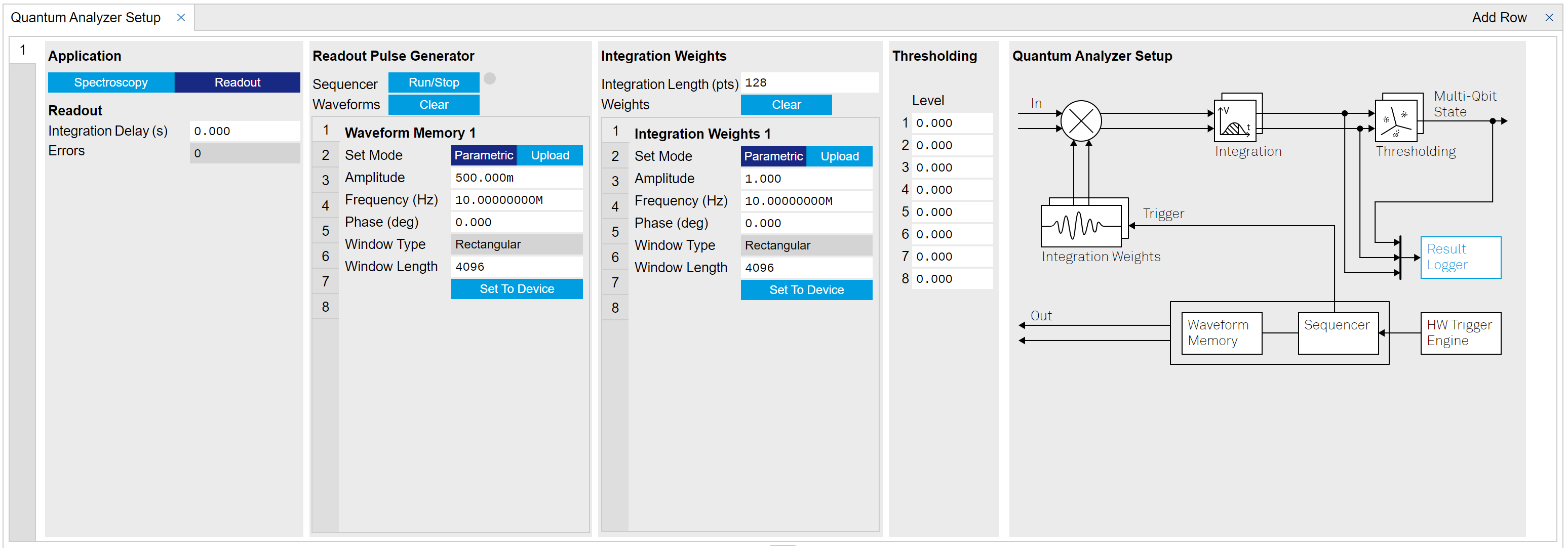
Readout mode is mainly used for multi qubit readout. The SHFQC+ has 8 or 16 readout Waveform Memory slots, and 8 or 16 integration weight units per Quantum Analyzer channel. In readout mode, these memory slots are used for readout pulse generation and weighted integration. The SHFQC+ Readout Pulse Generator is the central controller in Readout mode, see Figure 5 and tutorial Multiplexed Qubit Readout.

Figure 5: Readout waveform generation, integration and discrimination in Readout mode.

There are 2 state discrimination modes, 2-state discrimination (default, see tutorial Multiplexed Qubit Readout and multistate discrimination). Both modes are based on the linear Support Vector Machine and one versus one classification. Note that multistate discrimination can only be configured via LabOne APIs.

Readout Waveform Generation In Readout Mode¶

The readout waveform can be generated parametrically by LabOne GUI and APIs, and then uploaded and saved in the Waveform Memory. All readout waveforms saved in the Waveform Memory can be erased by clicking Clear on LabOne GUI or using LabOne APIs. Each readout waveform can be used for a single qudit readout, and up to 8 or 16 qubits can be readout simultaneously using a sum of the readout waveforms saved in the Waveform Memory. The Readout Waveform Generator controls which and how readout waveforms are played, see the Readout Pulse Generator Tab.

The readout waveform saved in the \(j\)-th (\(j\le\) 8 or 16) Waveform Memory slot is complex data, which can be expressed as

\[ \begin{equation}\tag{8} \begin{aligned} E_{i,\ j,\ \mathrm{readout}} & = A_{i,\ j,\ \mathrm{readout}}e^{i2\pi f_{j,\ \mathrm{offset}}t_{i} + i\phi_{j,\ \mathrm{readout}}} \end{aligned} \end{equation} \]

where \(A_{i,\ j,\ \mathrm{readout}}\ (0\le A_{i,\ j,\ \mathrm{readout}}\le 1)\) is the amplitude factor of the readout waveform at the \(i\)-th sample, \(f_{j,\ \mathrm{offset}}\) is the offset frequency, \(\phi_{j,\ \mathrm{readout}}\) is the global phase. The output signal on the front panel is

\[ \begin{equation}\tag{9} \begin{aligned} E_{\mathrm{output}}(t) & = \operatorname{Re}[\sum_j A_{j,\ \mathrm{readout}}(t)e^{i2\pi (f_{j,\ \mathrm{offset}}+f_0)t + i\phi_{j,\ \mathrm{readout}}}] \end{aligned} \end{equation} \]

where the sum depends on number of qudits readout in parallel. Note that the maximum amplitude factor of the sum of all waveforms in use should not exceed 1.

Integration Weights¶

The integration weights can be parametrically generated or measured with the SHFQC+ Scope for the best SNR (see tutorial Integration Weights Measurement), and uploaded to the integration weight units. All integration weights saved in the memory can be erased by clicking Clear on LabOne GUI Integration Weights sub-tab or using LabOne APIs. The length of the integration weight is automatically extended to 4096 Samples once it’s uploaded, and integration length is used to configure how long it integrates. The Readout Waveform Generator controls which and how integration weights are used, see Readout Pulse Generator Tab.

The integration weights saved in the \(k\)-th integration weight unit is complex data, can be expressed as

\[ \begin{equation}\tag{10} \begin{aligned} E_{i,\ k,\ \mathrm{weights}} & = A_{i,\ k,\ \mathrm{weight}}e^{-i2\pi f_{k,\ \mathrm{weight}}t_{i} - i\phi_{k,\ \mathrm{weight}}}, \end{aligned} \end{equation} \]

where \(A_{i,\ k,\ \mathrm{weight}}\ (0\le A_{i,\ k,\ \mathrm{weight}}\le 1)\) is the amplitude factor of the integration weight at \(i\)-th sample, \(f_{k,\ \mathrm{weight}}\) is the frequency of the integration weight, \(\phi_{k,\ \mathrm{weight}}\) is the global phase of the integration weight.

In 2-state discrimination mode, 1 qubit requires 1 integration weight, i.e. the conjugated difference of readout input signal while qubit is prepared in state |0> and |1>, see Figure 6. In multistate discrimination mode, 1 qudit with \(n\) states requires \(n(n-1)/2\) integration weighs (one vs one classification), i.e. the conjugated differences of any 2 readout input signal while qudit is prepared in state |\(i\)> and |\(j\)>, where \(i\ (0\le i\le n-2)\) and \(j\ (1\le j\le n-1)\) are integer and \(i \neq j\). Only \(n-1\) integration weights need to be uploaded, and the integration results from the rest of integration weights are calculated by the Instrument automatically, see Figure 7 and Figure 8.

All integration weights saved in the integration weight units can be displayed on the Waveform Viewer, see Figure 3.

Note

In order to achieve the highest possible resolution in the signal after integration, it’s advised to scale the dimensionless readout integration weights with a factor so that their maximum absolute value is equal to 1.

Thresholding¶

Thresholding sub-tab is used to configure thresholds for state discrimination in 2-state discrimination mode. In multistate discrimination mode, thresholds and assignment matrix are configured by LabOne APIs.

The input signal before integration is

\[ \begin{equation}\tag{11} \begin{aligned} E_{i,\ \mathrm{before\ integration}} = \begin{cases} C_{\mathrm{scaling}}\sum_j \frac{A_{i,\ j,\ \mathrm{input}}}{2}e^{i2\pi f_{j,\ \mathrm{baseband}}t_i+\phi_{j,\ \mathrm{input}}}, & \mathrm{RF\ path},\\\ C_{\mathrm{scaling}}\sum_j A_{i,\ j,\ \mathrm{input}}\cos{(2\pi f_{j,\ \mathrm{baseband}}t_i+\phi_{j,\ \mathrm{input}}}), & \mathrm{LF\ path}, \end{cases} \end{aligned} \end{equation} \]

where \(i\) indicates the \(i\)-th sample of the input signal, \(j\) indicates the \(j\)-th component of the input signal for a qubit or qudit, \(A_{i,\ j,\ \mathrm{input}}\) is the amplitude of \(j\)-th components of the input signal, \(f_{j,\ \mathrm{baseband}}\) is the frequency of \(j\)-th component of the input signal, \(\phi_{j,\ \mathrm{input}}\), is the phase of \(j\)-th component of input signal. The signal can be monitored by the SHFQC+ Scope with the same conversion factors as in Spectroscopy mode,

\[ \begin{equation}\tag{12} E_{\mathrm{Scope}} = \begin{cases} \Sigma_j\frac{A_{i,\ j,\ \mathrm{input}}}{\sqrt{2}}e^{i2\pi f_{j,\ \mathrm{baseband}} t_i + i\phi_{j,\ \mathrm{input}}}, & \mathrm{RF\ path,} \\\ \Sigma_j A_{i,\ j,\ \mathrm{input}}\cos{(2\pi f_{j,\ \mathrm{baseband}} t_i + \phi_{j,\ \mathrm{input}})}, & \mathrm{LF\ path.} \end{cases} \end{equation} \]

This signal is then integrated with integration weights \(A_{i,\ j,\ \mathrm{weight}}e^{-i2\pi f_{j,\ \mathrm{weight}}t_i-i\phi_{j,\ \mathrm{weight}}}\) (\(f_{j,\ \mathrm{weight}} = f_{j,\ \mathrm{baseband}}\)) simultaneously. The \(j\)-th integration result after weighted integration is

\[ \begin{equation}\tag{13} \begin{aligned} E_{j,\ \mathrm{after\ integration}} &= \Sigma_{i=1}^N {E_{i,\ j,\ \mathrm{before\ integration}}A_{i, j,\ \mathrm{weight}}e^{-i2\pi f_{j,\ \mathrm{baseband}}t_i-i\phi_{j,\ \mathrm{weight}}}}\\\ &= \begin{cases} \frac{C_{\mathrm{scaling}}}{2}\sum_{i=1}^N A_{i,\ j,\ \mathrm{input}}A_{i, j,\ \mathrm{weight}}e^{i(\phi_{j,\ \mathrm{input}}-\phi_{j,\ \mathrm{weight}})}, & \mathrm{RF\ path,}\\\ \frac{C_{\mathrm{scaling}}}{2}\sum_{i=1}^N A_{i,\ j,\ \mathrm{input}}A_{i, j,\ \mathrm{weight}}\times\\\ (e^{i(\phi_{j,\ \mathrm{input}}-\phi_{j,\ \mathrm{weight}})} + e^{-i 4 \pi f_{j,\ \mathrm{baseband}}t_i-i\phi_{j,\ \mathrm{weight}}-i\phi_{j,\ \mathrm{weight}}}), & \mathrm{LF\ path.} \end{cases} \end{aligned} \end{equation} \]

If \(\phi_{j,\ \mathrm{input}}=\phi_{j,\ \mathrm{weight}}\), \(A_{i,\ j,\ \mathrm{input}} = A_{j,\ \mathrm{input}}\) is a constant, \(A_{i,\ j,\ \mathrm{weights}} = 1\), and integration length is much longer than \(1/(2 f_{j,\ \mathrm{baseband}})\) with LF path, the result after integration can be simplified as \(E_{j,\ \mathrm{after\ integration}} = \frac{NC_{\mathrm{scaling}}A_{j,\ \mathrm{input}}}{2}\). This result with RF (LF) path is complex data, and can be downloaded and displayed on the Quantum Analyzer Result Tab with a conversion factor of \(\sqrt{2}/C_{\mathrm{scaling}}\) (\(1/C_{\mathrm{scaling}}\)), as \(\frac{NA_{j,\ \mathrm{input}}}{\sqrt{2}}\) (\(\frac{NA_{j,\ \mathrm{input}}}{2}\)).

To achieve the best SNR, the largest separation of qubit states and discriminate states with real data, one can apply optimal weights \((E_{j,\ |b\rangle,\ \mathrm{Scope}} - E_{j,\, |a\rangle,\ \mathrm{Scope}})^*/A_{\mathrm{norm}}\), where \(E_{j,\, |b\rangle,\ \mathrm{Scope}}\) (\(E_{j,\, |a\rangle,\ \mathrm{Scope}}\)) is the readout signal when qubit in state \(|b\rangle\) (\(|a\rangle\)) before integration recorded by the scope, "*" is a conjugate operation, \(A_{\mathrm{norm}}\) is a factor to normalize the optimal weights. The readout signal \(E_{|b\rangle\ ,\ \mathrm{after\ integration}}\) of a single qubit after weighted integration with the optimal weights is

\[ \begin{equation}\tag{14} \begin{aligned} &E\_{|b\rangle\ ,\ \mathrm{after\ integration}}\\\ &= \begin{cases} \frac{C\_{\mathrm{scaling}}}{2}\Sigma\_{i=1}^N\frac{A\_{i,\ |b\rangle}}{A'\_{i,\ \mathrm{norm}}}e^{i\phi\_{|b\rangle}}(A\_{i,\ |b\rangle}e^{i\phi\_{|b\rangle}} - A\_{i,\ |a\rangle}e^{i\pi\_{|a\rangle}})^*,& \mathrm{RF\ path},\\\ C\_{\mathrm{scaling}}\Sigma\_{i=1}^N\frac{A\_{i,\ |b\rangle}}{A''\_{i,\ \mathrm{norm}}}\cos{\phi\_{|b\rangle}}(A\_{i,\ |b\rangle}\cos{\phi\_{|b\rangle}} - A\_{i,\ |a\rangle}\cos{\phi\_{|a\rangle}}), & \mathrm{LF\ path}, \end{cases}\\\ &= \begin{cases} \frac{C\_{\mathrm{scaling}}}{2}\Sigma\_{i=1}^N\frac{A\_{i,\ |b\rangle}}{A'\_{i,\ \mathrm{norm}}}[A\_{i,\ |b\rangle}-A\_{i,\ |a\rangle}\cos{(\phi\_{|b\rangle}-\phi\_{|a\rangle})-i A\_{i,\ a}\sin{(\phi\_{|b\rangle}-\phi\_{|a\rangle})}}], & \mathrm{RF\ path},\\\ C\_{\mathrm{scaling}}\Sigma\_{i=1}^N\frac{A\_{i,\ |b\rangle}}{A''\_{i,\ \mathrm{norm}}}\cos{\phi\_{|b\rangle}}(A\_{i,\ |b\rangle}\cos{\phi\_{|b\rangle}} - A\_{i,\ |a\rangle}\cos{\phi\_{|a\rangle}}), & \mathrm{LF\ path}, \end{cases} \end{aligned} \end{equation} \]

where \(A'\_{i,\ \mathrm{norm}}=\sqrt{A\_{i,\ |b\rangle}^2+A\_{i,\ |a\rangle}^2-2 A\_{i,\ |a\rangle}A\_{i,\ |b\rangle}\cos{(\phi\_{|a\rangle}-\phi\_{|b\rangle})}}\) (\(A''\_{i,\ \mathrm{norm}}=A\_{i,\ |b\rangle}\cos{\phi\_{|b\rangle}} - A\_{i,\ |a\rangle}\cos{\phi\_{|a\rangle}}\)) is a normalization factor, \(A\_{i,\ |b\rangle}\) (\(A\_{i,\ |a\rangle}\)) and \(\phi\_{|b\rangle}\) (\(\phi\_{|a\rangle}\)) is the amplitude and phase of the signal in state \(|b\rangle\) (\(|a\rangle\)), respectively. Similarly, the readout signal \(E\_{|a\rangle\ ,\ \mathrm{after\ integration}}\) after weighted integration with the optimal weights is

\[ \begin{equation}\tag{15} \begin{aligned} &E\_{|a\rangle\ ,\ \mathrm{after\ integration}}\\\ &=\begin{cases} \frac{C\_{\mathrm{scaling}}}{2}\Sigma\_{i=1}^N\frac{A\_{i,\ |a\rangle}}{A'\_{i,\ \mathrm{norm}}}[-A\_{i,\ |a\rangle}+A\_{i,\ |b\rangle}\cos{(\phi\_{|a\rangle}-\phi\_{|b\rangle})+i A\_{i,\ |b\rangle}\sin{(\phi\_{|a\rangle}-\phi\_{|b\rangle})}}], & \mathrm{RF\ path},\\\ C\_{\mathrm{scaling}}\Sigma\_{i=1}^N\frac{A\_{i,\ |a\rangle}}{A''\_{i,\ \mathrm{norm}}}\cos{\phi\_{|a\rangle}}(A\_{i,\ |b\rangle}\cos{\phi\_{|b\rangle}} - A\_{i,\ |a\rangle}\cos{\phi\_{|a\rangle}}), & \mathrm{LF\ path}, \end{cases} \end{aligned} \end{equation} \]

Take the real part of the integrated results, and the 2 states can be discriminated by a threshold as

\[ \begin{equation}\tag{16} \begin{aligned} &\frac{\operatorname{Re}[E\_{|b\rangle\ ,\ \mathrm{after\ integration}}]+\operatorname{Re}[E\_{|a\rangle\ ,\ \mathrm{after\ integration}}]}{2}\\\ &=\begin{cases} \frac{C\_{\mathrm{scaling}}}{2}\Sigma\_{i=1}^N\frac{1}{A'\_{\mathrm{i,\ norm}}}(A\_{i,\ |b\rangle}^2 - A\_{i,\ |a\rangle}^2), & \mathrm{RF\ path},\\\ C\_{\mathrm{scaling}}\Sigma\_{i=1}^N\frac{1}{A''\_{\mathrm{i,\ norm}}}(A\_{i,\ |b\rangle}^2\cos^2{\phi\_{|b\rangle}} - A\_{i,\ |a\rangle}^2\cos^2{\phi\_{|a\rangle}}), & \mathrm{LF\ path}. \end{cases} \end{aligned} \end{equation} \]

The separation between state \(|b\rangle\) and state \(|a\rangle\) can be calculated directly as \(\sqrt{\Sigma\_{i=1}^N(A\_{i,\ |b\rangle}^2 + A\_{i,\ |a\rangle}^2-2 A\_{i,\ |a\rangle}A\_{i,\ |b\rangle}\cos{(\phi\_{|b\rangle}-\phi\_{|a\rangle})}})\), and it is the same as calculated from

\[ \begin{equation}\tag{17} \begin{aligned} |\operatorname{Re}[E_{|b\rangle\ ,\ \mathrm{after\ integration}}]-\operatorname{Re}[E_{|a\rangle\ ,\ \mathrm{after\ integration}}]|. \end{aligned} \end{equation} \]

In 2-state discrimination mode, all integration weights can be uploaded via LabOne GUI and APIs, and all integration results saved in the result logger can be displayed on the Quantum Analyzer Result Tab if integration is selected as result source. In multistate discrimination mode, all integration weights can only be uploaded via LabOne APIs, and only \(n-1\) integration results are saved in the result logger if integration is selected as result source, the rest are calculated automatically in the pairwise difference units.

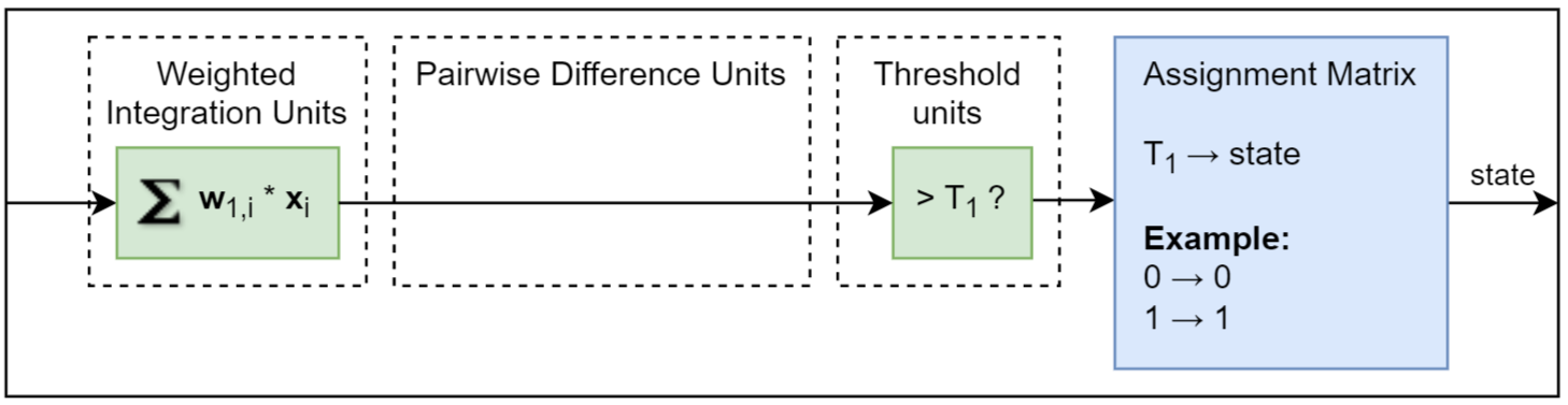
Before state discrimination, threshold \(T_j\) for each qudit has to be estimated and uploaded to the Instrument with an internal conversion factor \(\frac{2}{C_{\mathrm{scaling}}}\) (\(\frac{1}{C_{\mathrm{scaling}}}\)) in RF (LF) path. During thresholding, the real part of the result after integration is compared with a threshold, and it returns 0 or 1. Qubit state discrimination can be done in both 2-state and multistate discrimination modes. The readout result of qubit after thresholding is

\[ \begin{equation}\tag{18} \begin{aligned} E_{j,\ \mathrm{after\ thresholding}}= \begin{cases} 0 & \mathrm{Re}[E_{j,\ \mathrm{after\ integration}}] \le T_j,\\\ 1 & \mathrm{Re}[E_{j,\ \mathrm{after\ integration}}] \gt T_j, \end{cases} \end{aligned} \end{equation} \]

where \(T_j\) is the threshold of the \(j\)-th qubit, see Figure 6. The result after thresholding can represent qubit state directly.

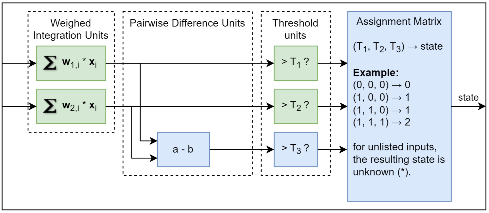
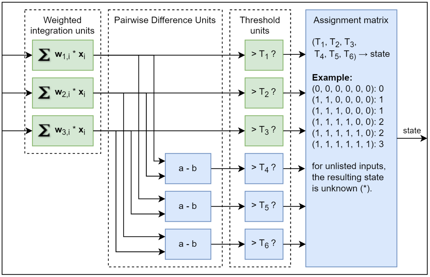
Figure 6: Readout data processing for qubits. The green blocks are used for both state discrimination modes and the blue blocks are used for multistate discrimination mode only configured by LabOne APIs. \(x_i\) is the readout input signal at the \(i\)-th sample, \(w_{1,\ i}\) is the optimal integration weight calculated from the difference while qubit is prepared in state |0> and |1>, \(T_1\) is the threshold for the integrated result.

For a qutrit, 3 thresholds are used, 2 for the integration results in the weighted integration units and 1 for the integration result in the pairwise difference units, see Figure 7. After thresholding, the 3-bit data is assigned to 0, 1 or 2 by the assignment matrix, and the discriminated results can be displayed in the Quantum Analyzer Result Tab. The discriminated result represented by 2-bit data can be transferred to control instruments via DIO and ZSync for feedback experiment.

Figure 7: Readout data processing for qutrits. The green blocks are used for both state discrimination modes and the blue blocks are used for multistate discrimination mode only configured by LabOne APIs. \(x_i\) is the readout input signal at the \(i\)-th sample,\(w_{1,\ i}\) and \(w_{2,\ i}\) are the integration weights measured by calculating the readout pulse difference when the qutrit is prepared in state |0> and |1>, and state |0> and |2>, respectively. "a - b" is the pairwise difference of the integration results. The pairwise difference is equivalent to having the third weighted integration \(\sum (w_{1,\ i} - w_{2,\ j}) \cdot x_i\). \(T_1\), \(T_2\) and \(T_3\) are the thresholds for the 3 integration results.

For a ququad, 6 thresholds are used, 3 for the integration results in the weighted integration units and 3 for the integration results in the pairwise difference units, see Figure 8. After thresholding, the 6-bit data is assigned to 0, 1, 2 or 3 by the assignment matrix, and the discriminated results can be displayed in the Quantum Analyzer Result Tab. The discriminated result represented by 2-bit data can be transferred to control instruments via DIO and ZSync for feedback experiment.

Figure 8: Readout data processing for ququads. \(x_i\) is the readout input signal at the \(i\)-th sample, \(w_{1,\ i}\), \(w_{2,\ i}\) and \(w_{3,\ i}\) are the integration weights measured by calculating the readout pulse difference when the ququad is prepared in state |0> and |1>, state |0> and |2>, and state |0> and |3>, respectively. "a - b" are the pairwise differences of the integration results. These pairwise differences are equivalent to having 3 more weighted integration \(\sum (w_{1,\ i} - w_{2,\ j}) \cdot x_i\), \(\sum (w_{1,\ i} - w_{3,\ j}) \cdot x_i\) and \(\sum (w_{2,\ i} - w_{3,\ j}) \cdot x_i\). \(T_1\), \(T_2\), \(T_3\), \(T_4\), \(T_5\) and \(T_6\) are the thresholds for 6 integration results.

Functional Elements¶

Table 5: QA setup settings
Control/Tool	Option/Range	Description
Application Mode	Spectroscopy	Using internal digital oscillator for waveform generation and integration.
Application Mode		Readout	Using uploaded waveform for output signal generation and customized weights for integration.
Errors	Number	Number of hold-off errors detected since last reset.
Spectroscopy
Trigger Signal		Selects the source of the trigger for the integration and envelope in Spectroscopy mode.
Integration Length	2^2 to 2^25	Sets the integration length in Spectroscopy mode in number of samples. Up to 33.5 MSa (2^25 samples, with granularity of 4 Samples ) can be recorded, which corresponds to 16.7 ms.
Integration Delay	-4 ns to 131.1 μs	Sets the delay of the integration in Spectroscopy mode with respect to the trigger signal. The resolution is 2 ns.
Operation Mode	Continuous	The output of the internal digital oscillator is used directly for frequency up-conversion.
Operation Mode		Pulse	The waveform envelope is modulated by the internal digital oscillator before frequency up-conversion.
Length	4 to 32 k (SHFQC+ without 16W option) or 64 k	Indicate the length of uploaded envelope waveform in units of Samples. The granularity is 4 Samples.
Delay	0 ns to 131.1 μs	Set a delay between readout pulse playback trigger and the first sample of the readout pulse (in Pulsed mode). The resolution is 2 ns.
File Upload	CSV file	Drop CSV file to upload the envelope waveform.
Center Frequency	RF: 1 - 8 GHz LF: 0 Hz	Display center frequency in Spectroscopy mode.
Offset Frequency	- 1 to +1 GHz	Set offset frequency to the internal digital oscillator in Spectroscopy mode.
Output Frequency	DC - 8.5 GHz	Display frequency of the output signal in Spectroscopy mode.
Amplitude	0 to 1	Set gain of the internal digital oscillator in Spectroscopy mode. The recommended range is from 0.01 to 1 in pulsed mode.
Readout
Integration Length	4 to 4096	Sets the length of all Integration Weights in number of samples. A maximum of 4096 samples can be integrated, which corresponds to 2.05 μs. The granularity is 4 Samples.
Integration Delay	0 ns to 131.1 μs	Sets a common delay for the start of the readout integration for all Integration Weights with respect to the time when the trigger is received. The resolution is 2 ns.
Sequencer Run/Stop	Run or Stop	Enables the Sequencer.
Waveforms Clear		Empty all readout Waveform Memory slots or Integration weight Units.
Waveform Generation	Parametric or Upload	Select the way to generate waveform.
Parametric Amplitude	0 to 1	Set amplitude factor for parametric readout pulse and integration weight generation.
Parametric Frequency	-1 to +1 GHz	Set offset frequency for parametric readout pulse or integration weight generation.
Parametric Phase	-180 to 180 degree	Set phase for parametric readout pulse and integration weight generation.
Parametric Window Type	Rectangular	Display window function to be applied in complex exponential function for parametric readout pulse and integration weight generation.
Parametric Window Length	4 to 4096	Length of the selected window in samples for parametric readout pulse and integration weight generation.
Parametric Set To Device	Yes or No	Set parametrically generated readout pulse and integration weight to waveform memory slot and integration memory slot, respectively.
Thresholding	-14.51 kV to 14.51 kV	Set threshold for quantum state discrimination. Note that the data before thresholding is not normalized by the integration length.