Basic Waveform Playback
Note
This tutorial is applicable to all SHFQC+ Instruments.
Goals and Requirements
The goal of this tutorial is to demonstrate the basic use of the Signal Generator channels of the SHFQC+, by demonstrating simple waveform generation and playback. In order to visualize the multi-channel signals, an oscilloscope with sufficient bandwidth and channel number is required. This can be an external scope, or the scope of the SHFQC+, for which a loopback configuration is needed with the Quantum Analyzer channel.
Preparation
Connect the cables as illustrated below. Make sure that the instrument is powered on and connected by Ethernet to your local area network (LAN) where the host computer resides. After starting LabOne, the default web browser opens with the LabOne graphical user interface.
Note
The instrument can also be connected via the USB interface, which can be simpler for a first test. As a final configuration for measurements, it is recommended to use the 1GbE interface, as it offers a larger data transfer bandwidth.

The tutorial can be started with the default instrument configuration (e.g. after a power cycle) and the default user interface settings (e.g. after pressing F5 in the browser).
Waveform Generation and Playback
In this tutorial we generate signals with the AWG and visualize them with the scope. In a first step we enable the Output of the Signal Generator channel of the SHFQC+ and set the Output Range. We also set the RF center frequency to 1 GHz. In this example, we will use the RF path, which supports center frequencies in the range 0.6 - 8 GHz. When using the LF path, the center frequency can be set in the range 0 - 2 GHz. Additionally, we configure the scope with a suitable time base (e.g. 500 ns per division) and range (e.g. 0.2 V per division). The following table summarizes the necessary settings.
| Tab | Sub-tab | Label | Setting / Value / State |
|---|---|---|---|
| In/Out | SG Channel 1 | On | ON |
| In/Out | SG Channel 1 | Range (dBm) | 10 |
| In/Out | SG Channel 1 | Center Freq (Hz) | 1.0 G |
| In/Out | SG Channel 1 | Output Path | RF |
| Scope Setting | Value / State |
|---|---|
| Ch1 enable | ON |
| Ch1 range | 0.2 V/div |
| Timebase | 500 ns/div |
| Trigger source | Ch1 |
| Trigger level | 200 mV |
| Run / Stop | ON |
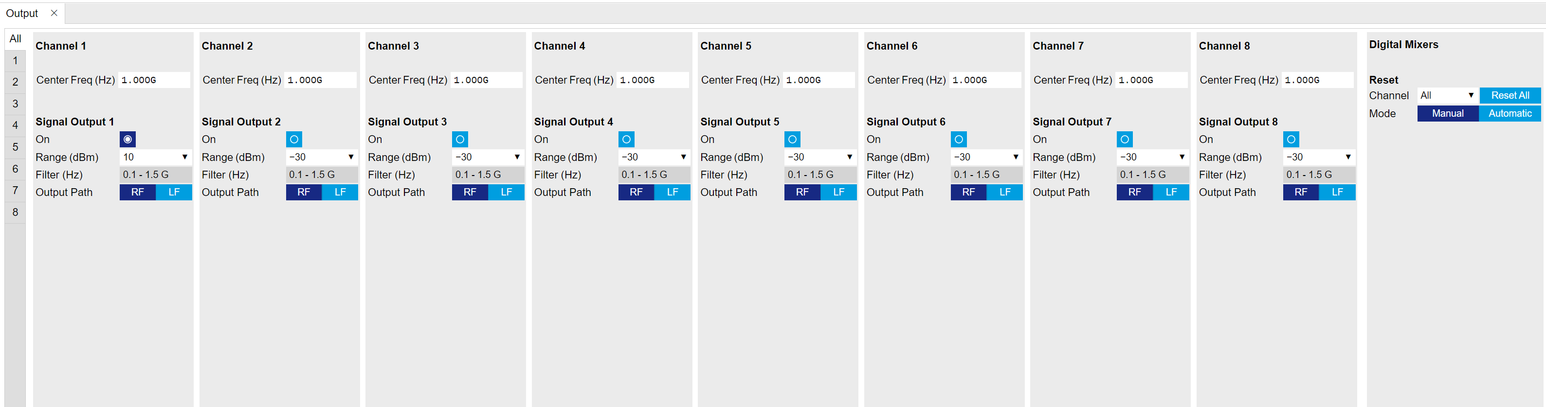
In the In/Out Tab, we configure the first Signal Generator output channel.
The final signal amplitude is determined by the dimensionless signal amplitude stored in the waveform memory scaled to the set Range in dBm of the channel. The necessary settings are summarized in the following table.
| Tab | Sub-tab | Section | # | Label | Setting / Value / State |
|---|---|---|---|---|---|
| AWG | Control | Sampling Rate | 2 GHz | ||
| Digital Modulation | Modulation Control | 1 | Modulation | OFF | |
| Digital Modulation | AWG Outputs | Amplitude | 1.0 |
To operate the AWG we need to specify a sequence program through a C-type language. This program is then compiled and uploaded to the instrument where it is executed in real time. Writing the sequence program can be done interactively by typing the program in the sequence window. Let’s start by typing the following code into the sequence editor.
wave w_gauss = 1.0*gauss(8000, 4000, 1000);
playWave(1, w_gauss);
In the first line of the program, we generate a waveform with a Gaussian
shape with a length of 8000 samples and store the waveform under the
name w_gauss. The peak center position 4000 and the standard deviation
1000 are both defined in units of samples. You can convert them into
time by dividing by the chosen Sampling Rate (2.0 GSa/s by default). The
waveform generated by the gauss function has a peak amplitude of 1.
This amplitude is dimensionless and the output amplitude of the physical
signal is given by this number multiplied with the voltage determined by
the selected output range (here we chose 0 dBm). To calculate the
maximum amplitude \(V_p\) in Volts use:
\(V_p=\sqrt{2 * 10^{P_\mathrm{max}/10} * 10^{-3} \,\mathrm{W} * 50\,\Omega}\),
where \(P_\mathrm{max}\) is the Range setting in dBm. \(V_p\) corresponds to
the peak voltage of a signal of a given power when connected to a
\(50\,\Omega\) load. To calculate he RMS amplitude \(V_{rms}\), divide by
\(\sqrt{2}\), i.e. \(V_{rms}=\frac{V_p}{\sqrt{2}}\). Of course, the scaling
factor of 1.0 in the waveform definition can be replaced by any other
value. Finally, the code line is terminated by a semicolon according to
C conventions.
With the second line of the program, the generated waveform w_gauss is
played on
the output of the first Signal Generator channel.
We use the
syntax playWave(1,w_gauss) to play a Gaussian signal in the real
quadrature of the complex output. For a more detailed discussion of how
the playWave command routes the AWG outputs to generate complex
signals, see the Digital Modulation
Tutorial. Note that the syntax of
the playWave command and the values of other parameters, such as the
waveform amplitude, can yield signals that are either below or above the
maximum output power. If a signal happens to be above the maximum output
power, it will clip at the DAC and may be distorted. For more details on
playWave and how different amplitude settings influence the final
signal, see the Modulation Tutorial.
Note
For this tutorial, we will keep the description of the Sequencer instructions short. You can find the full specification of the LabOne Sequencer language in LabOne Sequence Programming
Note
The AWG has a waveform granularity of 16 samples, and a minimum waveform
length of 32 samples when using playWave commands or 16 samples when
using the command table (see the Pulse-level Sequencing
Tutorial ). It’s recommended to use
waveform lengths that are multiples of 16, to avoid having ill-defined
samples between successively played waveforms. Waveforms that are not
multiple of 16 samples are automatically padded with 0s and a compiler
warning is issued.
By clicking on  ,
the sequence program is compiled into sequence instructions that are
then uploaded to the device together with the waveform data. A
successful upload is indicated by a green Compiler Status LED. Any error
that causes an upload failure of either the sequencer instruction or
waveform data is indicated by a red status light.
,
the sequence program is compiled into sequence instructions that are
then uploaded to the device together with the waveform data. A
successful upload is indicated by a green Compiler Status LED. Any error
that causes an upload failure of either the sequencer instruction or
waveform data is indicated by a red status light.
Note
The Advanced tab shows how the sequence instructions translate to assembly language for the onboard FPGA.
By clicking on the Waveform sub-tab, we see that our Gaussian waveform appeared in the list. The Memory Usage field at the bottom of the Waveform sub-tab shows what fraction of the instrument memory is filled by the waveform data. The Waveform Viewer sub-tab allows you to graphically display the currently marked waveform in the list.
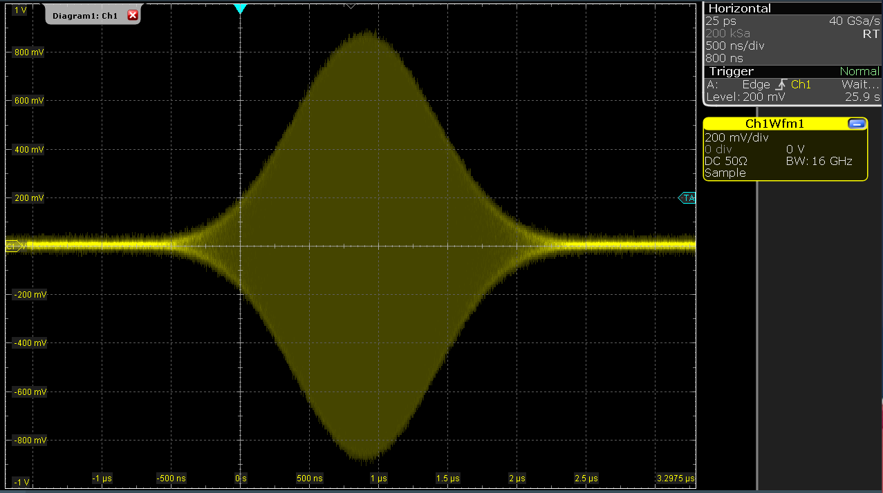
Clicking on  executes the uploaded AWG program. Since we have armed the scope
previously with a suitable trigger level, it has captured our Gaussian
pulse with a FWHM of about 1.5 μs and a carrier frequency of 1.0 GHz, as
shown in Figure Figure 3.
executes the uploaded AWG program. Since we have armed the scope
previously with a suitable trigger level, it has captured our Gaussian
pulse with a FWHM of about 1.5 μs and a carrier frequency of 1.0 GHz, as
shown in Figure Figure 3.
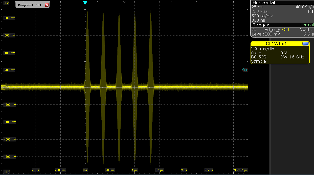
The LabOne Sequencer language offers various run-time control. An
important functionality, e.g. for real-time averaging of an experiment,
is the repetition of a sequence. In the following example, all the code
within the curly brackets {...} is repeated 5 times. Upon clicking
and ,
we observe 5 short Gaussian pulses in a new scope shot, see Figure 4.
wave w_gauss = 1.0 * gauss(640, 320, 50);

repeat (5) {
  playWave(1, w_gauss);
}
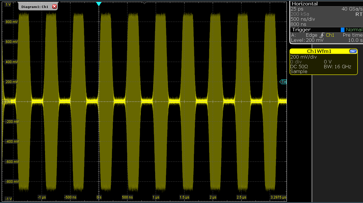
In order to generate more complex waveforms, the LabOne Sequencer
programming language offers a rich toolset for waveform manipulation. In
addition to a selection of standard waveform generation functions,
waveforms can be added, multiplied, scaled, concatenated, and truncated.
It’s also possible to use compile-time evaluated loops to generate pulse
series with systematic parameter variations – see LabOne Sequence
Programming
for more information. In the following code example, we make use of some
of these tools to generate a pulse with a smooth rising edge, a flat
plateau, and a smooth falling edge. We use the cut function to cut a
waveform at defined sample indices, the ones function to generate a
waveform with constant level 1.0 and length 320, and the join function
to concatenate three (or arbitrarily many) waveforms.
wave w_gauss = gauss(640, 320, 50);
wave w_rise = cut(w_gauss, 0, 319);
wave w_fall = cut(w_gauss, 320, 639);
wave w_flat = rect(320, 1.0);

wave w_pulse = join(w_rise, w_flat, w_fall);

while (true) {
  playWave(1, w_pulse);
}
Note that we replaced the finite repetition by an infinite repetition by
using a while loop. Loops can be nested in order to generate complex
playback routines. The output generated by the program above is shown in
Scope shot of an infinite pulse series generated by the
AWG.
As programs get longer, it becomes useful to store and recall them.
Clicking on  allows you to store the present program under a new name. Clicking on
then saves your program to the file name displayed at the top of the
editor. As you begin to work on sequence programs more regularly, it’s
worth using some of the editor keyboard shortcuts listed in Sequence
Editor Keyboard
Shortcuts.
allows you to store the present program under a new name. Clicking on
then saves your program to the file name displayed at the top of the
editor. As you begin to work on sequence programs more regularly, it’s
worth using some of the editor keyboard shortcuts listed in Sequence
Editor Keyboard
Shortcuts.
It’s also possible to iterate over the samples of a waveform array and
calculate each one of them in a loop over a compile-time variable
cvar. This often allows sequences to go beyond the possibilities of
using the predefined waveform generation function, particularly when
using nested formulas of elementary functions like in the following
example. The waveform array needs to be pre-allocated e.g. using the
instruction zeros.
const N = 1024;
const width = 100;
const position = N/2;
const f_start = 0.1;
const f_stop = 0.2;
cvar i;
wave w_array = zeros(N);
for (i = 0; i < N; i++) {
  w_array[i] = sin(10/(cosh((i-position)/width)));
}

playWave(w_array);
It is also possible to use waveforms stored as a list of values in a
file. If the file is stored in the location
(C:\Users\<user name>\Documents\Zurich Instruments\LabOne\WebServer\awg\waves\
under Windows or ~/Zurich Instruments/LabOne/WebServer/awg/waves/
under Linux), you can then play back the wave by referring to the file
name without extension in the sequence program:
playWave("wave_file");
If you prefer, you can also store it in a wave data type first and
give it a new name:
wave w = "wave_file";
playWave(w);
For more information about the file format, please refer to the AWG Module Section of the LabOne Programming Manual.
Using the LF Path
The LF path bypasses the upconversion chain to allow center frequencies in the range DC to 2 GHz to be generated. The AWG sequencer can be programmed in the same way as with the RF path. The main differences is that the maximum output power of the LF path is +5 dBm (compared to +10 dBm for the RF path) and that the latency of the LF path is shorter than that of the RF path, due to the shorter analog path.
The center frequency of the LF path can be set in multiples of 100 MHz. When combined with correct usage of waitDigTrigger and resetOscPhase commands, this ensures that the initial
phase of a played waveform will be reproducible within a given
experimental run, as in the following example:
const length = 128;
const amp = 1;
wave = gaussian(length, amp, length/2, length/8);

while (1) {
  waitDigTrigger(1);
  resetOscPhase();
  playWave(1, 2, wave);
}