Saving and Loading Data
Overview
In this section we discuss how to save and record measurement data with the SHFQC+ Instrument using the LabOne user interface. In the LabOne user interface, there are 3 ways to save data:
- Saving the data that is currently displayed in a plot
- Continuously recording data in the background
- Saving trace data in the History sub-tab
Furthermore, the History sub-tab supports loading data. In the following, we will explain these methods.
Saving Data from Plots
A quick way to save data from any plot is to click on the Save CSV icon
 at the bottom of the plot to store the currently displayed curves as a
comma-separated value (CSV) file to the download folder of your web
browser. Clicking on
will save a graphics file instead.
at the bottom of the plot to store the currently displayed curves as a
comma-separated value (CSV) file to the download folder of your web
browser. Clicking on
will save a graphics file instead.
Recording Data
The recording functionality allows you to store measurement data continuously, as well as to track instrument settings over time. The Config Tab gives you access to the main settings for this function. The Format selector defines which format is used: HDF5, CSV, or MATLAB. The CSV delimiter character can be changed in the User Preferences section. The default option is Semicolon.
The node tree display of the Record Data section allows you to browse
through the different measurement data and instrument settings, and to
select the ones you would like to record. For instance, the demodulator
1 measurement data is accessible under the path of the form
Device 0000/Demodulators/Demod 1/Sample. An example for an instrument
setting would be the filter time constant, accessible under the path
Device 0000/Demodulators/Demod 1/Filter Time Constant.
The default storage location is the LabOne Data folder which can, for
instance, be accessed by the Open Folder button  .
The exact path is displayed in the Folder field whenever a file has been
written.
.
The exact path is displayed in the Folder field whenever a file has been
written.
Clicking on the Record checkbox will initiate the recording to the hard drive.
In case HDF5 or MATLAB is selected as the file format, LabOne creates a single file containing the data for all selected nodes. For the CSV format, at least one file for each of the selected nodes is created from the start. At a configurable time interval, new data files are created, but the maximum size is capped at about 1 GB for easier data handling. The storage location is indicated in the Folder field of the Record Data section.
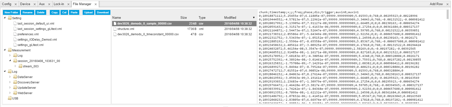
The File Manager Tab is a good place to inspect CSV data files. The file browser on the left of the tab allows you to navigate to the location of the data files and offers functionalities for managing files in the LabOne Data folder structure. In addition, you can conveniently transfer files between the folder structure and your preferred location using the Upload/Download buttons. The file viewer on the right side of the tab displays the contents of text files up to a certain size limit. Figure 1 shows the Files tab after recording Demodulator Sample and Filter Time Constant for a few seconds. The file viewer shows the contents of the demodulator data file.
Note
The structure of files containing instrument settings and of those containing streamed data is the same. Streaming data files contain one line per sampling period, whereas in the case of instrument settings, the file usually only contains a few lines, one for each change in the settings. More information on the file structure can be found in the LabOne Programming Manual.
History List
Tabs with a history list such as
Scope Tab,
support feature saving, autosaving, and loading functionality. By
default, the plot area in those tools displays the last 100 measurements
(depending on the tool, these can be sweep traces, scope shots, DAQ data
sets, or spectra), and each measurement is represented as an entry in
the History sub-tab. The button to the left of each list entry controls
the visibility of the corresponding trace in the plot; the button to the
right controls the color of the trace. [^1]Double-clicking on a list
entry allows you to rename it. All measurements in the history list can
be saved with  .
Clicking on the
.
Clicking on the  button (note the dropdown button
  )
saves only those traces that were selected by a mouse click. Use the
Control or Shift button together with a mouse click to select multiple
traces. The file location can be accessed by the Open Folder button
.
Figure 4.8 illustrates some of these features. Figure 2 illustrates the data loading feature.
)
saves only those traces that were selected by a mouse click. Use the
Control or Shift button together with a mouse click to select multiple
traces. The file location can be accessed by the Open Folder button
.
Figure 4.8 illustrates some of these features. Figure 2 illustrates the data loading feature.
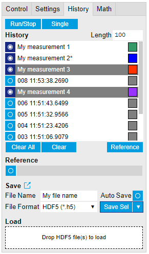
Which quantities are saved depends on which signals have been added to the Vertical Axis Groups section in the Control sub-tab. Only data from demodulators with enabled Data Transfer in the Lock-in tab can be included in the files.
The history sub-tab supports an autosave functionality to store
measurement results continuously while the tool is running. Autosave
directories are differentiated from normal saved directories by the text
"autosave" in the name, e.g. sweep_autosave_000. When running a tool
continuously ( button) with Autosave activated, after the current measurement (history
entry) is complete, all measurements in the history are saved. The same
file is overwritten each time, which means that old measurements will be
lost once the limit defined by the history Length setting has been
reached. When performing single measurements (
button) with Autosave activated, after the current measurement (history
entry) is complete, all measurements in the history are saved. The same
file is overwritten each time, which means that old measurements will be
lost once the limit defined by the history Length setting has been
reached. When performing single measurements ( button) with Autosave activated, after each measurement, the elements in
the history list are saved in a new directory with an incrementing
count, e.g.
button) with Autosave activated, after each measurement, the elements in
the history list are saved in a new directory with an incrementing
count, e.g. sweep_autosave_001, sweep_autosave_002.
Data which was saved in HDF5 file format can be loaded back into the
history list. Loaded traces are marked by a prefix "loaded " that is
added to the history entry name in the user interface. The
createdtimestamp information in the header data marks the time at
which the data were measured.
- Only files created by the Save button in the History sub-tab can be loaded.
- Loading a file will add all history items saved in the file to the history list. Previous entries are kept in the list.
- Data from the file is only displayed in the plot if it matches the current settings in the Vertical Axis Group section the tool. Loading e.g. PID data in the Sweeper will not be shown, unless it is selected in the Control sub-tab.
- Files can only be loaded if the devices saving and loading data are of the same product family. The data path will be set according to the device ID loading the data.
Figure 3 illustrates the data loading feature.

Supported File Formats
HDF5
Hierarchical Data File 5 (HDF5) is a widespread memory-efficient, structured, binary, open file format. Data in this format can be inspected using the dedicated viewer HDFview. HDF5 libraries or import tools are available for Python, MATLAB, LabVIEW, C, R, Octave, Origin, Igor Pro, and others. The following example illustrates how to access demodulator data from a sweep using the h5py library in Python:
import h5py
filename = 'sweep_00000.h5'
f = h5py.File(filename, 'r')
x = f['000/dev3025/demods/0/sample/frequency']
The data loading feature of LabOne supports HDF5 files, while it is unavailable for other formats.
MATLAB
The MATLAB File Format (.mat) is a proprietary file format from MathWorks based on the open HDF5 file format. It has thus similar properties as the HDF5 format, but the support for importing .mat files into third-party software other than MATLAB is usually less good than that for importing HDF5 files.
SXM
SXM is a proprietary file format by Nanonis used for SPM measurements.