Scope Tab
The Scope is a powerful time domain and frequency domain measurement tool as introduced in Unique Set of Analysis Tools and is available on all SHFQC+ Instruments.
Features
- Display complex signal in time domain
- 2 or 4 input channels with total memory of 64 kSa
- 14 bit nominal resolution
- Fast Fourier Transform (FFT) of complex signal: +/-500 MHz, spectral density and power conversion, choice of window functions
- Hardware Averaging up to 65536
- Segmented memory for up to 1024 scope shots
- Access internal triggers
Description
The Scope tab serves as the graphical display for time domain data. Whenever the tab is closed or an additional one of the same type is needed, clicking the following icon will open a new instance of the tab.
| Control/Tool | Option/Range | Description |
|---|---|---|
| Scope | Displays shots of data samples in time and frequency domain (FFT) representation. |
The Scope tab consists of a plot section on the left and a configuration section on the right. The configuration section is further divided into a number of sub-tabs. It gives access to a single-channel oscilloscope that can be used to monitor a choice of signals in the time or frequency domain. Hence the X axis of the plot area is time (for time domain display, Figure 1) or frequency (for frequency domain display, Figure 2). It is possible to display the time trace and the associated FFT simultaneously by opening a second instance of the Scope tab.
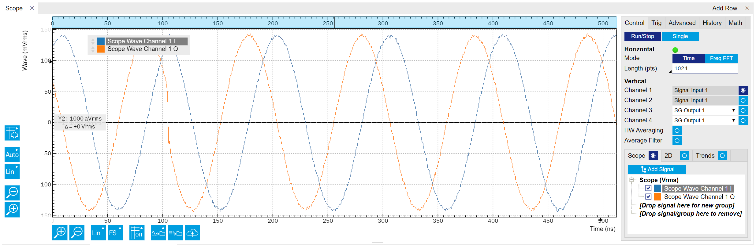
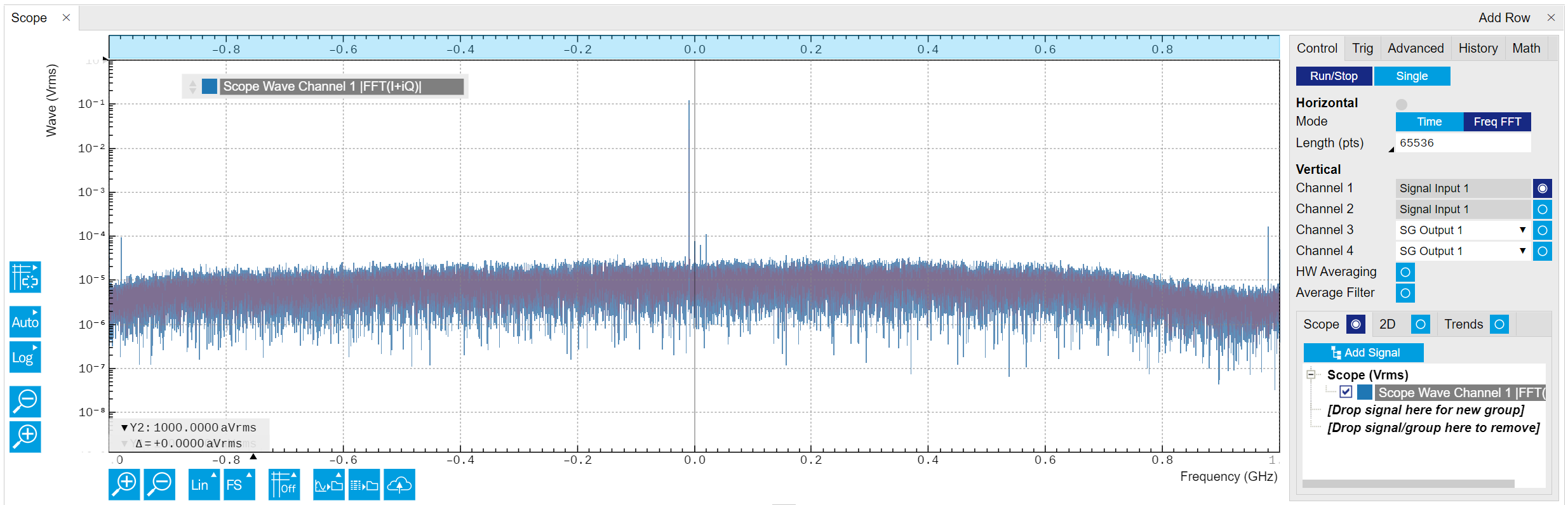
The raw complex data recorded by the Scope with a sampling rate of 2.0 GSa/s is from frequency down-conversion of the input signal, the Center Frequency is set in the Inputs/Outputs Tab. In the time-domain, the complex data is decomposed into 2 traces representing the real and imaginary components, respectively. With LF path, the imaginary components of the raw data is 0. For detailed data processing, please refer to Quantum Analyzer Setup Tab. The signal displayed in the FFT mode is calculated as \(|FFT(I+iQ)|\), where \(I\) is the real component of the complex data, and \(Q\) is the imaginary component. The frequency of input signal can be read as \(f_0 + f_{\mathrm{offset}}\), where \(f_0\) is the center frequency of the channel, and \(f_{\mathrm{offset}}\) is the offset frequency in the FFT plot. When using LF path, the FFT of input signal shows 2 sidebands \(\pm f_{\mathrm{offset}}\) around \(f_0 = 0\) since the input signal has real components only.
The Averaging function of the Scope mode is performed in the hardware level. This means if the number of averages is \(\gt1\), the recorded raw data is the data after the averaging, i.e. in the time-domain, the result is \(\langle I + i Q\rangle\), in FFT mode, the result is \(|FFT(\langle I+iQ \rangle)|\).
Functional Elements
| Control/Tool | Option/Range | Description |
|---|---|---|
| Run/Stop | Runs the scope/FFT with a default internal trigger (200 ms) if Trigger mode is disabled, or a configured trigger if Trigger mode is enabled. | |
| Single | Acquires a single shot of samples. | |
| Horizontal Mode | Time Domain / Freq Domain (FFT) | Switches between time and frequency domain display. |
| Shown Trigger | grey/green/yellow | When flashing, indicates that new scope shots are being captured and displayed in the plot area. The Trigger must not necessarily be enabled for this indicator to flash. A disabled trigger is equivalent to continuous acquisition. Scope shots with data loss are indicated by yellow. Such an invalid scope shot is not processed. |
| Length Mode & Value | Switches between length and duration display. | |
| Length (pts) 16 to \(2^{16}\) / \(2^{15}\) / \(2^{14}\) Sa for 1 / 2 / 3 or 4 channels; |
The scope shot length is defined in number of samples. The duration is given by the number of samples divided by the sampling rate 2.0 GSa/s. The granularity is 16 Samples. | |
| Duration (s) 8 ns to 32 / 16 / 8 \(\mu\)s for 1 / 2 / 3 or 4 channels; |
The scope shot length is defined as a duration. The number of samples is given by the duration times the sampling rate 2.0 GSa/s. The resolution is 8 ns. | |
| Channel N | Signal Input m (m is 1 to 2 or 1 to 4) | Select input source of the Scope channels. |
| Enable | ON / OFF | Activates the display of the corresponding scope channel. |
| Enable Hardware Averaging | ON / OFF | Enable hardware averaging where results are available and displayed only once all necessary shots have been acquired. As opposed to the EMA filter, the source data for hardware averaging is always the time trace before any postprocessing such as FFT. |
| Averages (HW) | 1 to 65536 | Number of shots to average on the Instrument before returning the data |
| Enable Average Filter | ON / OFF | Enable Exponential Moving Average (EMA) filter that is applied when the average of several scope shots is computed and displayed. Depending on the mode, the source data for averaging is either the Time or the Freq FFT trace. |
| Averages (EMA) | Integer from 1 | Number of shots required to reach 63% setting. Twice the number of shots yields 86% setting. |
| Reset (EMA) | Resets the averaging filter. | |
| Scope Display | ON / OFF | Display traces in a 1D plot. |
| 2D Display | ON / OFF | Display traces in a 2D plot. In segment mode, the vertical axis shows the number of segments, the horizontal axis shows the length/duration of the shots. It can be used together with Scope Display. |
| Trends Display | ON / OFF | Display trends of monitored traces. It can be used together with the Scope Display. |
| Control/Tool | Option/Range | Description |
|---|---|---|
| Enable | ON / OFF | When triggering is enabled scope shots are acquired every time the defined trigger condition is met. If disabled, scope shots are acquired continuously (every 200 ms). |
| Signal | Trigger Input nA and nB, Sequencer n Trigger Out, Sequencer n Monitor, Software Trigger, internal trigger. n is from 1 to 2 or 1 to 4 | Selects the trigger source signal. |
| Delay (s) | -4 \(\mu\)s to 131 \(\mu\)s | Trigger position relative to reference. A positive delay results in less data being acquired before the trigger point, a negative delay results in more data being acquired before the trigger point. The delay resolution is 2 ns. |
| Enable Segments | ON / OFF | Enable segmented scope recording. This allows for full bandwidth recording of scope shots with a minimum dead time between individual shots. |
| Segments | 1 to 1024 | Specifies the number of segments to be recorded in device memory. The maximum scope length size is given by the available memory divided by the number of segments. |
| Shown Trigger | 1 to 1024 | Displays the number of triggered events since last start. |
| Control/Tool | Option/Range | Description |
|---|---|---|
| FFT Window | Rectangular Hann Hamming Blackman Harris Exponential (ring-down) Cosine (ring-down) Cosine squared (ring-down) |
Seven different FFT windows to choose from. Each window function results in a different trade-off between amplitude accuracy and spectral leakage. Please check the literature to find the window function that best suits your needs. |
| Resolution (Hz) | 8 / 15 / 30 kHz to 125 MHz for 1 / 2 / 3 or 4 channels | Spectral resolution defined by the reciprocal acquisition time (sample rate, number of samples recorded). |
| Spectral Density | ON / OFF | Calculate and show the spectral density. If power is enabled the power spectral density value is calculated. The spectral density is used to analyze noise. |
| Power | ON / OFF | Calculate and show the power value. To extract power spectral density (PSD) this button should be enabled together with Spectral Density. |
| Persistence | ON / OFF | Keeps previous scope shots in the display. The color scheme visualizes the number of occurrences at certain positions in the time and amplitude by a multi-color scheme. |
| Control/Tool | Option/Range | Description |
|---|---|---|
| History | History | Each entry in the list corresponds to a single trace in the history. The number of traces displayed in the plot is limited to 20. Use the toggle buttons to hide or show individual traces. Use the color picker to change the color of a trace in the plot. Double click on a list entry to edit its name. |
| Length | 0 to 4294967295 | Maximum number of records in the history. The number of entries displayed in the list is limited to the 100 most recent ones. |
| Clear All | Remove all records from the history list. | |
| Clear | Remove selected records from the history list. | |
| Save | Save the traces in the history to a file accessible in the File Manager tab. The file contains the signals in the Vertical Axis Groups of the Control sub-tab. The data that is saved depends on the selection from the pull-down list. Save All: All traces are saved. Save Sel: The selected traces are saved. | |
| File Name | Enter a name which is used as the head of the folder name to save the history into. An additional three-digit counter is added as the rest of the folder name automatically to identify consecutive files. | |
| File Format | Select the file format in which to save the data. | |
| Auto Save | Activate autosaving. When activated, any measurements already in the history are saved. Each subsequent measurement is then also saved. The autosave directory is identified by the text "autosave" in the name, e.g. "sweep_autosave_001". If autosave is active during continuous running of the module, each successive measurement is saved to the same directory. For single shot operation, a new directory is created containing all measurements in the history. Depending on the file format, the measurements are either appended to the same file, or saved in individual files. For HDF5 and ZView formats, measurements are appended to the same file. For MATLAB and SXM formats, each measurement is saved in a separate file. | |
| Load file | Load data from a file into the history. Loading does not change the data type and range displayed in the plot, this has to be adapted manually if data is not shown. |