Integration Weights Measurement
Note
This tutorial is applicable to all SHFQC+ Instruments and no additional instrumentation is needed.
Goals and Requirements
LabOne Q is the recommended control software to operate the SHFQC+ for Quantum Technology applications.
The goal of this tutorial is to demonstrate how to use the SHFQC+ Scope to measure integration weights that are needed for high-fidelity single-shot readout using the LabOne User Interface (UI) and Zurich Instruments Toolkit API.
For qubit control with the SHFSG+ Signal Generator, the SHFQC+ Qubit Controller and the HDAWG Arbitrary Wave Generator, and instrument synchronization and feedback with the PQSC Programmable Quantum System Controller, see tutorials in the Online Documentation.
Note
For zhinst-toolkit users, please find the example in https://github.com/zhinst/zhinst-toolkit/blob/main/examples/shfqa_qubit_readout_weights.md, and the zhinst-toolkit documentation.
For LabOne Q users, please find the example in https://github.com/zhinst/laboneq/blob/main/examples/01_qubit_characterization/12_readoutweight_calibration_shfsg_shfqa_shfqc.ipynb, and the LabOne Q User Manual.
Preparation
Please follow the preparation steps in Connecting to the Instrument and connect the instrument in a loopback configuration as shown in Figure 1 or to a device under test.

Tutorial
In the tutorial, readout signals are recorded while the qubit is in ground and excited state. The readout pulse is generated by the SHFQC+ Readout Pulse Generator, and the signal recording is done by the SHFQC+ Scope. The integration weight is derived from the difference of the recorded readout signals.
This section shows how to use LabOne UI to configure the instrument, run the measurement, monitor the measurement results and calculate the integration weight.
-
Configure the instrument
-
Set center frequency and power range of input and output signals
Configure these parameters on the Input and Output Tab as in Figure 2 and in Table 1.
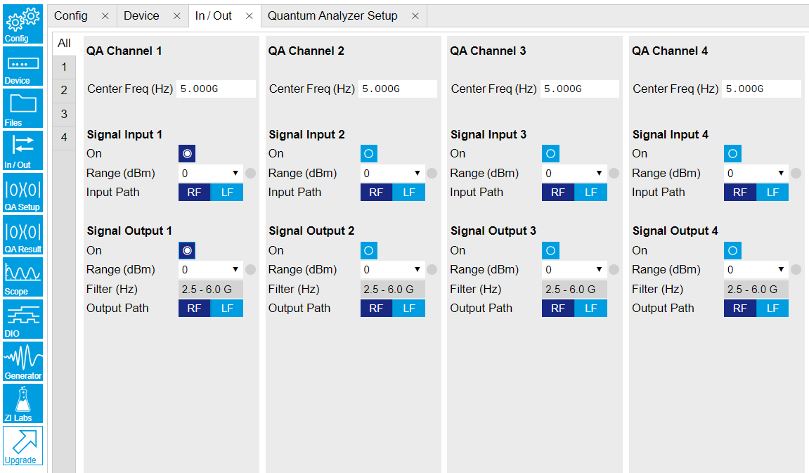
Figure 2: Configurations on In/Out Tab. Table 1: Settings of QA Channel 1 on In/Out Tab Parameter Setting Description QA Channel Selection All Select All to display all Channels. Cent Freq (Hz) 5 GHz Set center frequency of the frequency sweep of QA Channel 1. Signal Input 1 On Enable Enable the Signal Input 1. Signal Input 1 Range (dBm) 0 dBm Set power range of Signal Input 1 to 0 dBm. This setting allows the instrument to acquire a input signal with a power up to 0 dBm. Signal Input 1 Input Path RF Set input path of Signal Input 1 to RF path. Signal Output 1 On Enable Enable the Signal Output 1. Signal Output 1 Range 0 dBm Set power range of Signal Output 1 to 0 dBm. This setting allows the instrument to output a signal with a power up to 0 dBm. Signal Output 1 Output Path RF Set output path of the Signal Output 1 to RF path. -
Upload and compile measurement sequence
The measurement sequence is defined on the Sequence Sub-Tab of the Readout Pulse Generator Tab, see Table 2.
Table 2: Settings of QA Channel 1 on Readout Pulse Generator Tab. Parameter Setting Description QA channel Selection 1 Select QA channel 1. Sub-Tab Display Sequence Select Sequence sub-tab and paste the sequence program below. The Waveform Viewer sub-tab displays waveforms saved in Waveform Memory slots and Integration Weight units. Compile Click "To Device" Compile the sequence program by clicking "To Device". Digital Triggers Digital Trigger 1 Select Digital Trigger 1. Digital Trigger 1 Signal Internal Trigger Select Internal Trigger as the trigger source of Digital Trigger 1. Return Disable Disable return function. Run/Stop Enable Run the sequence. Below is the the sequence program for the measurement. In the loop, the
waitDigTriggercommand waits a trigger (see Table 3) to continue the sequence, thestartQAcommand sends a trigger to generate output waveform and start integration, it also sends a Sequencer Monitor Trigger (third argument of thestartQAcommand) to trigger SHFQC+ Scope to record input signal before integration. The measurement is repeated 100 times to get averaged readout pulses according to qubit prepared in ground and excited state.// repeat sequence 100 times, i.e. readout qubit in group state and excited state, and then repeat this 50 times repeat (100) { // wait for a trigger over ZSync. Assume the trigger period is longer than the cycle time // waitZSyncTrigger(); // alternatively wait for a trigger from digital trigger 1 waitDigTrigger(1); // play readout waveform stored in Waveform Memory slot 1, send a trigger to start integration, and send a Sequencer Monitor trigger to trigger the Scope startQA(QA_GEN_0, QA_INT_0, true); }The digital trigger set on the Trigger sub-tab is Internal Trigger. The configuration of the internal is shown in Table 3.
Table 3: Settings of Internal Trigger on DIO Setup Tab, see details on DIO Tab Parameter Setting Description Repetitions 100 Set number of repetitions. Holdoff (s) 100u Set holdoff time to 100 \(\mu\)s. Synchronization Disabled Disable Synchronization. Run/Stop Disable Disable the internal trigger. -
Configure signal generation
Signal generation is defined on QA Setup Tab, see Figure 3 and Table 4. Since we are only interested in the signal before integration, the settings for integration weights is not needed.
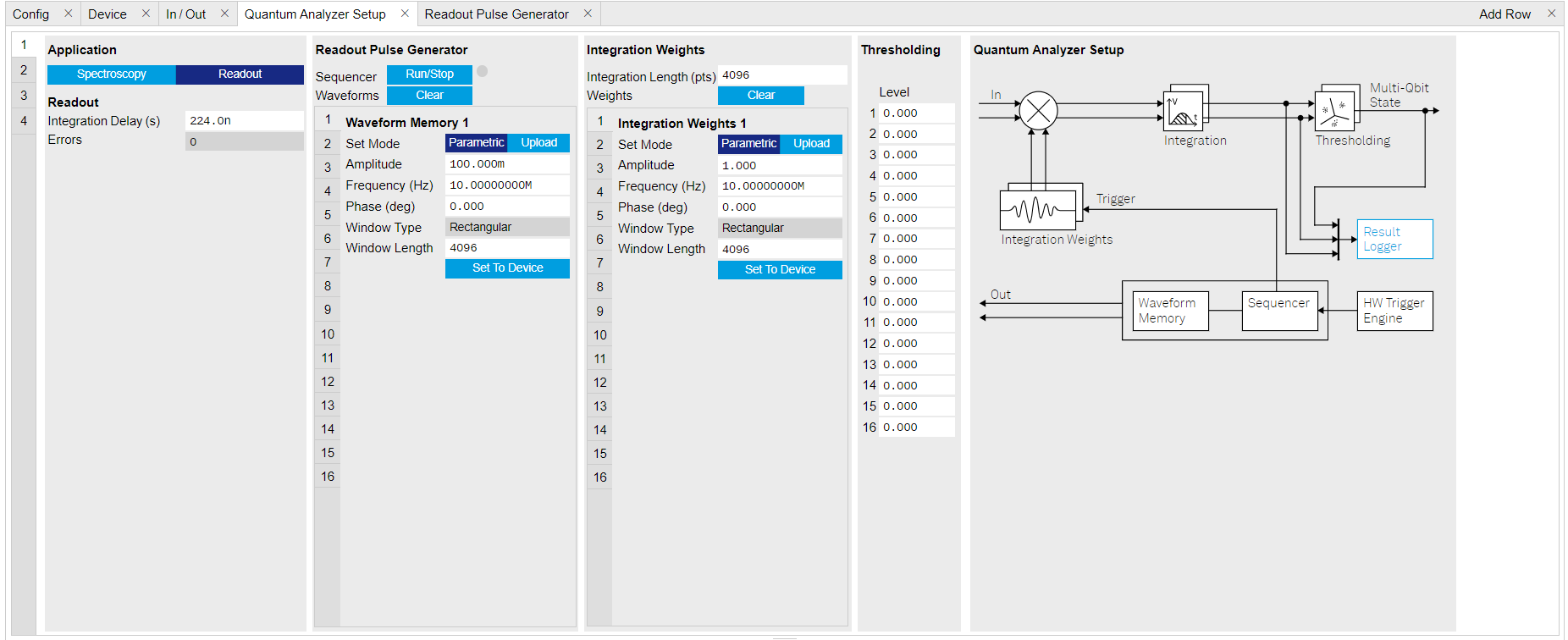
Figure 3: Configurations on QA Setup Tab. Table 4: Settings of QA Channel 1 on QA Setup Tab. Parameter Setting Description QA Channel Selection 1 Select QA Channel 1. Application Mode Readout Use Readout mode for integration weight measurement. Clear Waveform Click "Clear" Clear all waveforms saved in Waveform Memory. Clear all waveforms before uploading new ones to avoid incorrect waveform generation or output overflow. Waveform Memory 1 Set Mode Parametric Generate waveform parametrically in Waveform Memory slot 1. The parametrically generated waveform is \(Ae^{i (2 \pi f t + \frac{\pi}{180}\phi)}\), where \(A\) is the dimensionless amplitude factor of the waveform, \(f\) is the frequency in units of Hz, \(\phi\) is the phase in units of degree. Amplitude 0.5 Set amplitude factor \(A\) to 0.5. Frequency (Hz) 10M Set readout frequency \(f\) to 10 MHz. Phase (Deg) 0 Set phase \(\phi\) to 0 degree. Window Length 4096 Set length of the readout waveform in number of samples. Set To Device click "Set To Device" Upload the parametrically generated waveform to Waveform Memory slot 1. -
Configure SHFQC+ Scope
The SHFQC+ Scope is configured to record readout pulses before integration, and display averaged readout pulses according to qubit in ground state and excited state, see Figure 4 and Table 5. The figure shows the SHFQA+ Scope configuration for the same measurementNote that the input sources of the first and the second Scope channel are fixed to "Signal Input 1", and only SG channels can be selected as the input sources of the third and the forth Scope channel.
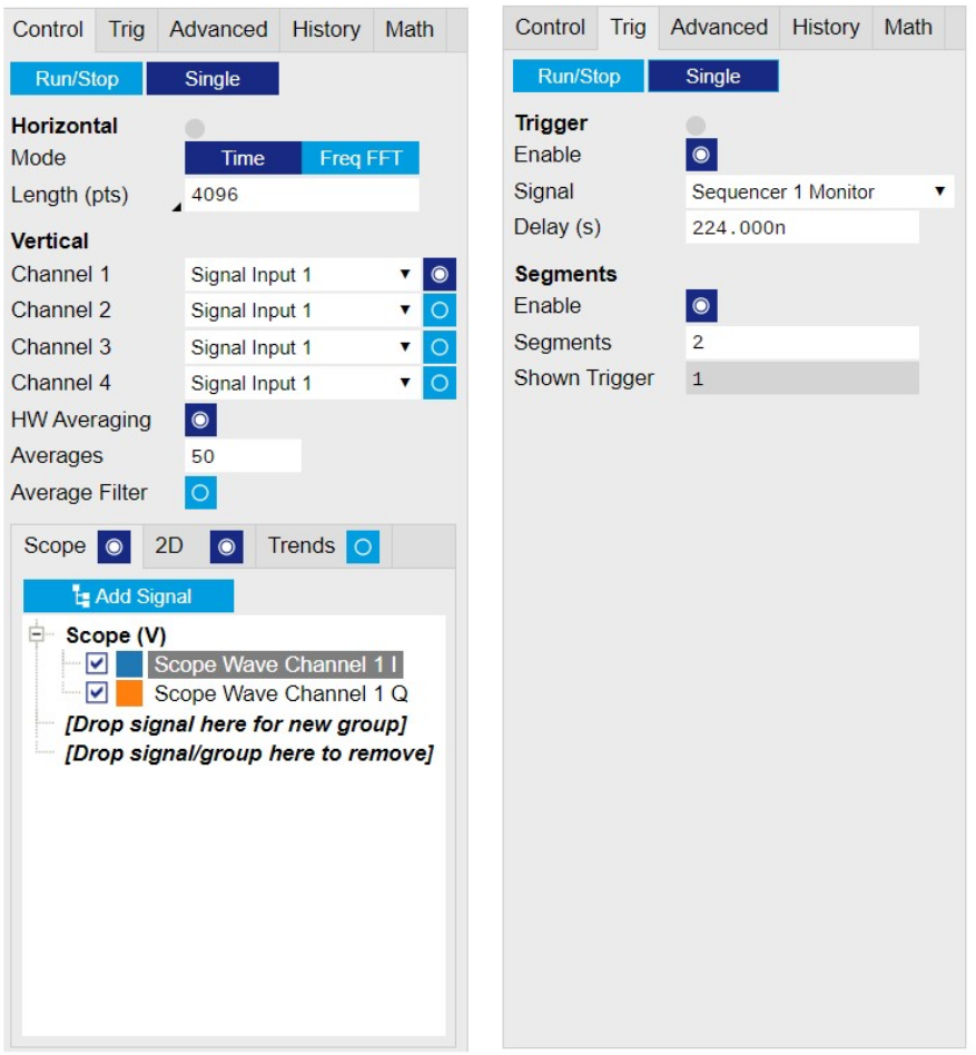
Figure 4: Configurations on Scope Tab. Table 5: Settings on Scope Tab Parameter Setting Description Horizontal Mode Time Display data in time-domain. Horizontal Length (pts) 4096 Set recording length in number of samples. This setting has to be \(\ge\) readout pulse length. Channel 1 Signal Selection Signal Input 1 Monitor signal comes from Signal Input 1 on Scope Channel 1. Channel 1 Enable Enable Enable Scope Channel 1. HW Averaging Enable Enable hardware averaging. Averages 50 Set number of averages to 50. This setting matches what is defined in the sequence program. Display Mode Scope Display the Scope trace. Enable "2D" if 2D trace is desired. Add Signal Scope Wave Channel 1 I and Q Add Scope Wave Channel 1 I and Scope Wave Channel 1 Q to the plot. Trigger Mode Enable Enable trigger mode so that scope recording starts only after receiving a trigger. Trigger Signal Sequencer 1 Monitor Trigger Select Sequencer 1 Monitor Trigger as the trigger to trigger the Scope. Trigger Delay (s) 224n Set trigger delay to 224 ns. The Scope starts to record data 224 ns later after receiving a trigger. This setting must has to match signal propagation delay including internal delay about 224 ns and external delay depending on the signal path between the front panel Signal Output port and Signal Input port. Segments Enable Enable Enable Segments measurement. In Segments measurement, the scope records \(n \times m\) data, where \(n\) is the number of segments, \(m\) is the recording length in number of samples. Segments 2 Set number of segments to 2. 1 for recording readout pulse when qubit in groud state, another for qubit in excited state. Run Mode Single Using Single mode for the measurement.
-
-
Run the measurement
By clicking "Run/Stop" icon on the System Settings sub-tab of DIO tab, the measurement is started and finished in seconds.
-
Monitor the measurement results and calculate the integration weight
The recorded readout pulses are displayed on the Scope Tab, as shown in Figure 5. The integration weights is calculated by taking the difference of the measured traces according to the qubit is in ground state and excited state.
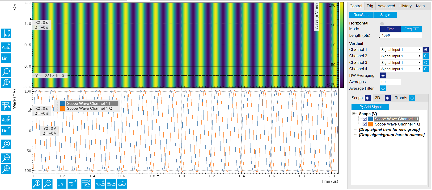
Figure 5: Recorded readout pulses on Scope Tab.
-
Connect the instrument
Create a toolkit session to the data server and connect the device with the device ID, e.g. 'DEV12001', see Connecting to the Instrument.
# Load the LabOne API and other necessary packages from zhinst.toolkit import Session, SHFQAChannelMode, Waveforms from scipy.signal import gaussian import numpy as np DEVICE_ID = 'DEVXXXXX' SERVER_HOST = 'localhost' session = Session(SERVER_HOST) ## connect to data server device = session.connect_device(DEVICE_ID) ## connect to device -
Generate readout pulses
In the tutorial, the envelope of the readout waveforms is flat-top Gaussian with pulse length of 500 ns and rise and fall time of 10 ns, amplitude factor of 0.9, and 8 readout frequencies span from 32 MHz to 120 MHz. The amplitude factor is not scaled by the number of qubits as in Multiplexed Qubit Readout because the readout output signal is generated from one of the readout waveforms, see the sequence program in the following section. The zhinst-toolkit class
Waveformsis for converting waveform data written in Python to data that can be uploaded to the instrument correctly.NUM_QUBITS = 8 SAMPLING_FREQUENCY = 2e9 RISE_FALL_TIME = 10e-9 PULSE_DURATION = 500e-9 rise_fall_len = int(RISE_FALL_TIME * SAMPLING_FREQUENCY) pulse_len = int(PULSE_DURATION * SAMPLING_FREQUENCY) std_dev = rise_fall_len // 10 gauss = gaussian(2 * rise_fall_len, std_dev) flat_top_gaussian = np.ones(pulse_len) flat_top_gaussian[0:rise_fall_len] = gauss[0:rise_fall_len] flat_top_gaussian[-rise_fall_len:] = gauss[-rise_fall_len:] # Scaling flat_top_gaussian *= 0.9 readout_pulses = Waveforms() time_vec = np.linspace(0, PULSE_DURATION, pulse_len) for i, f in enumerate(np.linspace(2e6, 32e6, NUM_QUBITS)): readout_pulses.assign_waveform( slot=i, wave1=flat_top_gaussian * np.exp(2j * np.pi * f * time_vec) ) -
Configure the channel
Configure center frequency, input and output power range and application mode of the channel using
qachannels[n].configure_channel, turn on the Input and Output, and upload the readout waveforms usinggenerator.write_to_waveform_memory.# configure inputs and outputs CHANNEL_INDEX = 0 # physical Channel 1 device.qachannels[CHANNEL_INDEX].configure_channel( center_frequency=5e9, # in units of Hz input_range=0, # in units of dBm output_range=-5, # in units of dBm mode=SHFQAChannelMode.READOUT, # SHFQAChannelMode.READOUT or SHFQAChannelMode.SPECTROSCOPY ) device.qachannels[CHANNEL_INDEX].input.on(1) device.qachannels[CHANNEL_INDEX].output.on(1) # write waveforms to the Waveform Memory device.qachannels[CHANNEL_INDEX].generator.write_to_waveform_memory(readout_pulses) -
Configure the Scope
Configure the Scope to record 2 segments of data with length of 500 ns which are averaged 50 times using
scopes[n].configure. The trigger of the Scope is1 Sequencer 1 Monitor Trigger which is enabled by thestartQAcommand.SCOPE_CHANNEL = 0 RECORD_DURATION = 500e-9 # in units of second NUM_SEGMENTS = 2 NUM_AVERAGES = 50 NUM_MEASUREMENTS = NUM_SEGMENTS * NUM_AVERAGES SAMPLING_FREQUENCY = 2e9 # in units of Hz device.scopes[0].configure( input_select={SCOPE_CHANNEL: f"channel{CHANNEL_INDEX}_signal_input"}, num_samples=int(RECORD_DURATION * SAMPLING_FREQUENCY), trigger_input=f"channel{CHANNEL_INDEX}_sequencer_monitor0", # Sequencer 1 monitor trigger num_segments=NUM_SEGMENTS, num_averages=NUM_AVERAGES, trigger_delay=214e-9, # record the data 214 ns later after receiving a trigger ) -
Configure and run the measurement, and calculate the integration weights
In the measurement, the Sequencer is triggered by Internal Trigger using
configure_sequencer_trigger.The integration weights for different qubits are measured sequentially with the
forloop. In each loop, theseqc_programis different and is uploaded to the instrument usingload_sequencer_program, both Scope and Sequencer run in Single mode set byscopes[n].runandenable_sequencerrespectively, the Generator sends 100 pulses to readout 1 of the qubits prepared in ground and excited state, and the Scope acquires 2 segments of data which are averaged 50 times, and the data is downloaded usingscopes[n].read, and integration weights are calculated in the end.results = [] device.qachannels[CHANNEL_INDEX].generator.configure_sequencer_triggering( aux_trigger=8,# internal trigger play_pulse_delay=0, # 0s delay between startQA trigger and the readout pulse ) device.system.internaltrigger.repetitions(int(NUM_SEGMENTS * NUM_AVERAGES)) device.system.internaltrigger.holdoff(100e-6) for i in range(NUM_QUBITS): qubit_result = { 'weights': None, 'ground_states': None, 'excited_states': None } print(f"Measuring qubit {i}.") # upload sequencer program seqc_program = f""" repeat({NUM_MEASUREMENTS}) {{ waitDigTrigger(1); startQA(QA_GEN_{i}, 0x0, true, 0, 0x0); // only QA_GEN_{i} matters for this measurement }} """ device.qachannels[CHANNEL_INDEX].generator.load_sequencer_program(seqc_program) # Start a measurement device.scopes[SCOPE_CHANNEL].run(single=True) device.qachannels[CHANNEL_INDEX].generator.enable_sequencer(single=True) device.system.internaltrigger.enable(1) # get results to calculate weights and plot data scope_data, *_ = device.scopes[0].read() # Calculates the weights from scope measurements # for the excited and ground states split_data = np.split(scope_data[SCOPE_CHANNEL], 2) ground_state_data = split_data[0] excited_state_data = split_data[1] qubit_result['ground_state_data'] = ground_state_data qubit_result['excited_state_data'] = excited_state_data qubit_result['weights'] = np.conj(excited_state_data - ground_state_data) results.append(qubit_result)The following code snippet can be used to plot readout traces (Figure 6) and calculate integration weights (Figure 7) of the last qubit.
Note
In order to achieve the highest possible resolution in the signal after integration, it’s advised to scale the dimensionless readout integration weights with a factor so that their maximum absolute value is equal to 1.
import matplotlib.pyplot as plt

fig, (ax0, ax1) = plt.subplots(nrows = 2, sharex = True)

t = np.linspace(0, RECORD_DURATION, int(RECORD_DURATION * SAMPLING_FREQUENCY/16)*16)
ax0.plot(t/1e-9, ground_state_data.real, '-', label = f'real')
ax0.plot(t/1e-9, ground_state_data.imag, '-', label = f'imag')
ax1.plot(t/1e-9, excited_state_data.real, '-', label = f'real')
ax1.plot(t/1e-9, excited_state_data.imag, '-', label = f'imag')

ax0.set_title('Ground state')
ax1.set_title('Excited state')
ax0.legend(loc='upper right')
ax1.legend(loc='upper right')
ax0.set_ylabel('Amplitude (Vrms)')
ax1.set_ylabel('Amplitude (Vrms)')
ax1.set_xlabel(r'Time (ns)')
plt.tight_layout()

plt.figure()
plt.plot(t/1e-9, results[0]['weights'])
plt.xlabel('Time (ns)')
plt.ylabel('Amplitude (Vrms)')
plt.tight_layout()
Figure 6: Readout pulses recorded by the Scope in loopback configuration 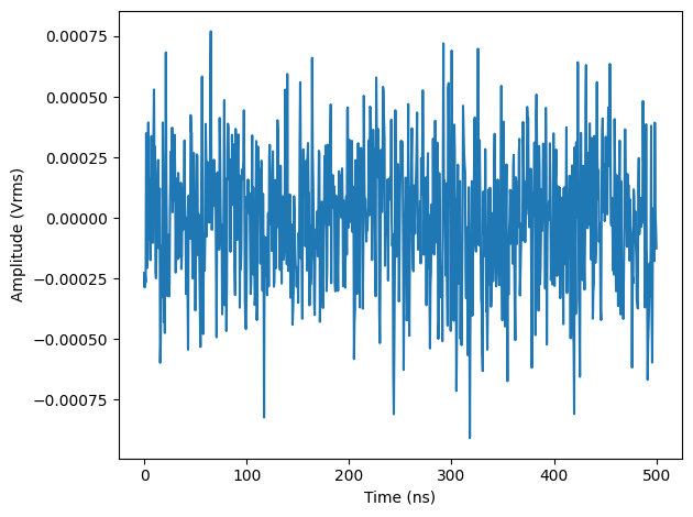
Figure 7: Integration weights calculated from the readout pulses