Pulse-level Sequencing with the Command Table

Note

This tutorial is applicable to all SHFQC+ Instruments.

Goals and Requirements

Pulse-level sequencing is an efficient way to encode pulses in a sequence by uploading a minimal amount of information to the device, allowing measurements to be performed more quickly and programmed more intuitively. The goal of this tutorial is to demonstrate pulse-level sequencing using the command table feature of the Signal Generator channels of theSHFQC+.

Preparation

Connect the cables as illustrated below. Make sure that the instrument is powered on and connected by Ethernet to your local area network (LAN) in which the control computer resides. After starting LabOne, the default web browser opens with the LabOne graphical user interface.

Figure 1: Connections for the arbitrary waveform generator command table tutorial

The tutorial can be started with the default instrument configuration (e.g. after a power cycle) and the default user interface settings (e.g. after pressing F5 in the browser). Additionally, this tutorial requires the use of one of our APIs, in order to be able to define and upload the command table itself. The examples shown here use the Python API - for an introduction see also the Python tutorial. Similar functionality is also available for other APIs.

Note

The instrument can also be connected via the USB interface, which can be simpler for a first test. As a final configuration for measurements, it is recommended to use the 1GbE interface, as it offers a larger data transfer bandwidth.

Configure the Output

Note

This tutorial makes use of the Zurich Instruments Toolkit. Setting a node in the Toolkit uses the format "device.path.to.node(value)." For the base Python API core, the equivalent node setting would be daq.set(f'/{DEVICE_ID}/path/to/node', value).

Note

The minimum waveform length when using the command table is 16 samples.

To begin with, we configure the output and digital modulation settings of the SHFQC+, to be able to observe our signal on a scope. We use the Zurich Instruments Toolkit, available in Python, to set the corresponding nodes after connecting to the instrument. The code below establishes a connection to the device before setting the node values (see also the Using the Python API Tutorial).

## Load the LabOne API and other necessary packages
from zhinst.toolkit import Session, CommandTable

DEVICE_ID = 'DEVXXXXX'
SERVER_HOST = 'localhost'

### connect to data server
session = Session(SERVER_HOST)

### connect to device
device = session.connect_device(DEVICE_ID)

SG_CHAN_INDEX = 0 # which channel to be used, here: first channel

##determine which synthesizer is used by the desired channel
synth = device.sgchannels[SG_CHAN_INDEX].synthesizer()

with device.set_transaction():
    # RF output settings
    device.sgchannels[SG_CHAN_INDEX].output.range(10) #output range in dBm
    device.sgchannels[SG_CHAN_INDEX].output.rflfpath(1) #use RF path, not LF path
    device.synthesizers[synth].centerfreq(1.0e9) #set the corresponding synthesizer frequency in Hz
    device.sgchannels[SG_CHAN_INDEX].output.on(1) #enable output
    # Digital modulation settings
    device.sgchannels[SG_CHAN_INDEX].awg.outputamplitude(0.5) #set the amplitude for the AWG outputs
    device.sgchannels[SG_CHAN_INDEX].oscs[0].freq(10.0e6) #frequency of oscillator 1 in Hz
    device.sgchannels[SG_CHAN_INDEX].oscs[1].freq(-150.0e6) #frequency of oscillator 2 in Hz
    device.sgchannels[SG_CHAN_INDEX].awg.modulation.enable(1) #enable digital modulation
    # Triggering settings
    device.sgchannels[SG_CHAN_INDEX].marker.source(0) #AWG trigger 1

In this case, we will use Signal Generator output channel 1 with a maximum output power of 10 dBm and an RF center frequency of 1.0 GHz. We will also enable digital modulation using an oscillator frequency of 10 MHz. This will yield a final output frequency of 1.01 GHz after configuring upper sideband modulation with the command table later. The amplitude of the AWG outputs is set to 0.5 to avoid saturating the outputs.

Introduction to the Command Table

The command table allows the sequencer to group waveform playback instructions with other timing-critical phase and amplitude setting commands into a single instruction that executes within one sequencer clock cycle of 4 ns. The command table is a unit separate from the sequencer and waveform memory and can thus be exchanged separately. Both the phase and the amplitude can be set in absolute and in incremental modes. Additionally, the active oscillator can be set with the command table, enabling fast, phase-coherent frequency switching on a given output channel. Even when not using digital modulation or amplitude settings, working with the command table has the advantage of being more efficient in sequencer instruction memory compared to standard sequencing. Starting a waveform playback with the command table always requires just a single sequencer clock cycle, as opposed to 2 or 3 when using a playWave instruction.

When using the command table, three components play together during runtime to generate the waveform output and apply the phase and amplitude setting instructions:

• Sequencer: the unit executing the runtime instructions, namely in this context the executeTableEntry instruction. This instruction executes one entry of the command table, and its input argument is a command table index. In its compiled form, which can be seen in the AWG Advanced sub-tab, the sequence program can contain up to 32768 instructions.
• Wave table: a list of up to 16000 indexed waveforms. This list is defined by the sequence program using the index assignment instruction assignWaveIndex combined with a waveform or waveform placeholder. The wave table index referring to a waveform can be used in two ways: it is referred to from the command table, and it is used to directly write waveform data to the instrument memory using the node <DEVICE_ID>/SGCHANNELS/<SG_CHAN_INDEX>/AWG/WAVEFORM/WAVES/<WAVE_INDEX> Node Documentation
• Command table: a list of up to 4096 indexed entries (command table index), each containing the index of a waveform to be played (wave table index), a sine generator phase setting, a set of four AWG amplitude settings for complex modulation, and an oscillator index selection. The command table is specified by a JSON formatted string written to the node <DEVICE_ID>/SGCHANNELS/<SG_CHAN_INDEX>/AWG/COMMANDTABLE/DATA

Basic command table use

We start by defining a sequencer program that uses the command table.

seqc_program = """\
// Define waveform
wave w_a = gauss(2048, 1, 1024, 256);

// Assign a single channel waveform to wave table entry 0
assignWaveIndex(1,2, w_a, 0);

// Reset the oscillator phase
resetOscPhase();

// Trigger the scope
setTrigger(1);
setTrigger(0);

// execute the first command table entry
executeTableEntry(0);
// execute the second command table entry
executeTableEntry(1);
"""

## Upload sequence
device.sgchannels[SG_CHAN_INDEX].awg.load_sequencer_program(seqc_program)

The sequence can be compiled and uploaded via API using the methods shown in the Python API Tutorial. The sequence defines a Gaussian pulse of unit amplitude and length of 2048 samples. This waveform is then assigned as a dual-channel waveform with explicit output assignment to the wave table entry with index 0, and the final lines execute the two first command table entries. This program cannot be run yet, as the command table is not yet defined.

Note

If a sequence program contains a reference to a command table entry that has not been defined, or if a command table entry refers to a waveform that has not been defined, the sequence program can’t be run.

In general the command table is defined as a JSON formatted string. Below, we show an example of how to define a command table with two table entries using Python. For ease of programming, here we define the command table as a CommandTable object, which is converted into a JSON string automatically at upload. Such object also validate the fields of the command table.

## Load CommandTable class
from zhinst.toolkit import CommandTable

## Initialize command table
ct_schema = device.sgchannels[SG_CHAN_INDEX].awg.commandtable.load_validation_schema()
ct = CommandTable(ct_schema)

## Index of wave table and command table entries
TABLE_INDEX = 0
WAVE_INDEX = 0
gain = 1.0

## Waveform with amplitude and phase settings
ct.table[TABLE_INDEX].waveform.index = WAVE_INDEX
ct.table[TABLE_INDEX].amplitude00.value = gain
ct.table[TABLE_INDEX].amplitude01.value = -gain
ct.table[TABLE_INDEX].amplitude10.value = gain
ct.table[TABLE_INDEX].amplitude11.value = gain
ct.table[TABLE_INDEX].phase.value = 0

## Same waveform with different amplitude and phase settings
ct.table[TABLE_INDEX+1].waveform.index = WAVE_INDEX
ct.table[TABLE_INDEX+1].amplitude00.value = gain/2
ct.table[TABLE_INDEX+1].amplitude01.value = -gain/2
ct.table[TABLE_INDEX+1].amplitude10.value = gain/2
ct.table[TABLE_INDEX+1].amplitude11.value = gain/2
ct.table[TABLE_INDEX+1].phase.value = 180

In this example, we generate a first command table entry with index "TABLE_INDEX", which plays the waveform referenced in the wave table at index "WAVE_INDEX", with amplitude and phase settings specified. The four amplitude settings of the command table have the same effect as the four gain settings of the Digital Modulation Tutorial, with analogous naming convention, i.e. amplitude01 maps to Gain01. The signs of the amplitudes are chosen to yield upper sideband modulation when using a positive oscillator frequency.

Note

Here we use a single-channel waveform, since we modulate only the amplitude of our pulses. Therefore, coefficients amplitude01 and amplitude11 are not strictly needed. We left them here and in the following examples to show how to use it even with dual-channel waveforms.

To upload the command table to the Signal Generator channel of the SHFQC+, we need to connect to the device and then write the command table to the correct node. In Python, this is achieved as follows:

## Upload command table
device.sgchannels[SG_CHAN_INDEX].awg.commandtable.upload_to_device(ct)

Note

During compilation of a sequencer program, any previously uploaded command table is reset, and will need to be uploaded again before it can be used.

Now that we’ve uploaded both the sequence and the command table, we can run the sequence:

device.sgchannels[SG_CHAN_INDEX].awg.enable_sequencer(single = True)

The expected output is shown in Figure 2. Note how the amplitude of the second waveform is half the magnitude of the first waveform, and that there is a phase shift of 180 degrees between them. This is due to the amplitude and phase settings in the command table. Also note that these amplitude settings are persistent. If a value is not explicitly specified in the command table, it uses either the default value or the value set by a previous usage of the 'executeTableEntry' instruction.

Figure 2: Output of the first channel from the basic command table example

Note

When a command table entry is called, the amplitude and phase are set persistently. Subsequent waveform playbacks on the same channel will need to take this into account, unless the amplitude and phase settings are explicitly included for them in their corresponding command table entries. Additionally, the values of the command table amplitude and phase settings take precedence over the corresponding gain and phase node settings set via API or in the LabOne UI, e.g. the value of Gain01 will have no effect if amplitude01 is specified in the command table entry.

Efficient pulse incrementation

One illustrative use case of the command table feature is the efficient incrementation of the amplitude or phase of a waveform.

We again start by writing a sequencer program that plays two entries of the command table.

seqc_program = """\
// Define a single waveform
wave w_a = ones(1024);

// Assign a single channel waveform to wave table entry
assignWaveIndex(1,2, w_a, 0);

// Reset the oscillator phase
resetOscPhase();

// Trigger the scope
setTrigger(1);
setTrigger(0);

// execute the first command table entry
executeTableEntry(0);
repeat(20) {
  executeTableEntry(1);
}
"""

## Upload sequence
device.sgchannels[SG_CHAN_INDEX].awg.load_sequencer_program(seqc_program)

Here we have defined a single wave table entry, where both channels contain the same constant waveform.

In Python we then define a command table with just two entries, in this case both referencing the same waveform index. In the second command table entry, we set the increment field to true, such that the amplitude is incremented each time that the second command table entry is called in the sequence.

## Initialize command table
ct_schema = device.sgchannels[SG_CHAN_INDEX].awg.commandtable.load_validation_schema()
ct = CommandTable(ct_schema)

## Waveform with initial amplitude
ct.table[0].waveform.index = 0
ct.table[0].amplitude00.value = 0
ct.table[0].amplitude01.value = 0
ct.table[0].amplitude10.value = 0
ct.table[0].amplitude11.value = 0

## Waveform with incremented amplitude
ct.table[1].waveform.index = 0
ct.table[1].amplitude00.value = 0.05
ct.table[1].amplitude01.value = -0.05
ct.table[1].amplitude10.value = 0.05
ct.table[1].amplitude11.value = 0.05
ct.table[1].amplitude00.increment = True
ct.table[1].amplitude01.increment = True
ct.table[1].amplitude10.increment = True
ct.table[1].amplitude11.increment = True

## Upload command table
device.sgchannels[SG_CHAN_INDEX].awg.commandtable.upload_to_device(ct)
## Enable sequencer
device.sgchannels[SG_CHAN_INDEX].awg.enable_sequencer(single = 1)

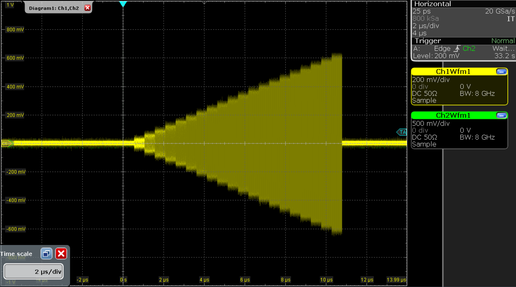
After uploading the command table to the instrument and executing the sequencer program, the channel then produces the output shown in Figure 3. Here, the first call to the first command table entry plays the waveform with all amplitude settings set to 0. The subsequent calls to the second command table entry increment these amplitudes each time by 0.05, with a negative increment on amplitude01, and a positive increment on the others. Although in this example we increment all amplitudes together, it is possible to increment only a subselection of the amplitude settings as well, by changing the appropriate increment settings to False. Incrementing amplitudes this way enables waveform memory-efficient amplitude sweeps.

Figure 3: Incrementing waveform amplitudes using the command table increment functionality

Note

The amplitude of the waveform generated at the output can be influenced in several different ways: through the amplitude of the waveform itself, through the amplitude settings in the command table, through the output amplitude setting in the Modulation Tab, and finally through the Range setting of the SHFQC+ Signal Generator output channel.

It is possible to perform multi-dimensional amplitude sweeps by making use of the amplitude registers of the command table. Each channel has four independent amplitude registers (indexed [0...3]), with each register storing the amplitude last played on that register. By default, amplitude register with index zero is used. It is therefore possible to keep the amplitude of one register constant while sweeping the amplitude of another register. This can be useful for probing dynamics in a multi-level system.

As an example, we will use the following sequence:

seqc_program = """\
//Constant definitions
const readout = 512; //length of readout in samples

//Waveform definition
wave wI1 = gauss(128, 1, 64, 16);
wave wI2 = gauss(256, 1, 128, 32);

//Assign index and outputs
assignWaveIndex(1,2,wI1,0);
assignWaveIndex(1,2,wI2,1);

var i = 10;
executeTableEntry(0);
do {
  executeTableEntry(2);
  executeTableEntry(1);
  playZero(readout);
  i-=1;
} while(i);
"""

# Upload sequence
device.sgchannels[SG_CHAN_INDEX].awg.load_sequencer_program(seqc_program)

The first executeTableEntry command initializes the amplitude that will be swept without playing a pulse. The second executeTableEntry plays a constant-amplitude Gaussian pulse (128 samples long). The third executeTableEntry plays a different Gaussian pulse (256 samples long), the amplitude of which will be swept. The loop will play 10 different amplitudes. We also need to define and upload a command table to go with the sequence:

# Initialize command table
ct_schema = device.sgchannels[0].awg.commandtable.load_validation_schema()
ct = CommandTable(ct_schema)

# Initialize amplitude register 1
ct.table[0].amplitude00.value = 0.0
ct.table[0].amplitude00.increment = False
ct.table[0].amplitude10.value = 0.0
ct.table[0].amplitude10.increment = False
ct.table[0].amplitudeRegister = 1

# Swept Gaussian pulse
ct.table[1].waveform.index = 1
ct.table[1].amplitude00.value = 0.05
ct.table[1].amplitude00.increment = True
ct.table[1].amplitude10.value = 0.05
ct.table[1].amplitude10.increment = True
ct.table[1].amplitudeRegister = 1

# Constant Gaussian pulse
ct.table[2].waveform.index = 0
ct.table[2].amplitude00.value = 0.9
ct.table[2].amplitude10.value = 0.9
ct.table[2].amplitudeRegister = 0

# Upload command table
device.sgchannels[SG_CHAN_INDEX].awg.commandtable.upload_to_device(ct)

The first command table entry (index 0) sets the initial amplitude (in this case, 0.0) of amplitude register 1. The second table entry (index 1) increments the amplitude of amplitude register 1 and plays the Gaussian pulse with waveform index 1. The third table entry (index 2) plays the constant-amplitude Gaussian pulse (waveform index 0) using amplitude register 0.

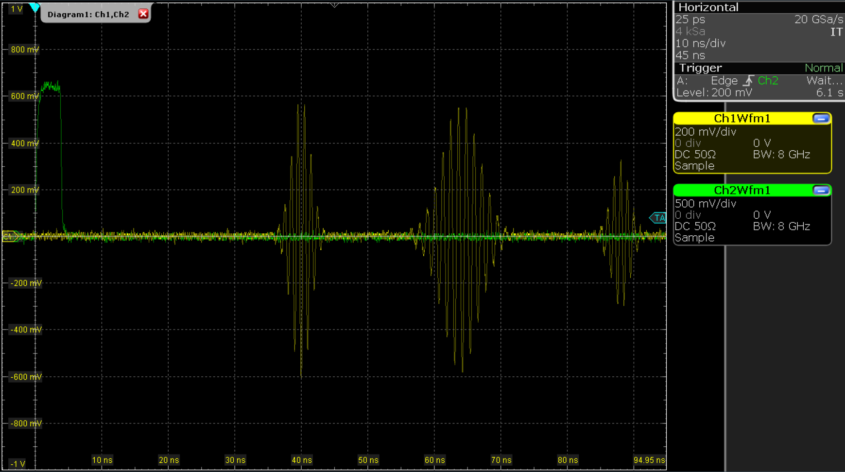
We now run the sequence:

device.sgchannels[SG_CHAN_INDEX].awg.enable_sequencer(single = 1)

We observe the signal shown in the figure below, which shows a constant-amplitude Gaussian pulse interleaved with a Gaussian pulse who amplitude is swept. In total, there are 10 different amplitudes of the swept pulse.

Figure 4: Using the amplitude registers to sweep the amplitude of one pulse while keeping the amplitude of another constant.

Phase sweeps can be achieved in a similar way by using the command table below.

## Define command table
## Initialize command table
ct_schema = device.sgchannels[SG_CHAN_INDEX].awg.commandtable.load_validation_schema()
ct = CommandTable(ct_schema)

## Waveform with initial phase
ct.table[0].waveform.index = 0
ct.table[0].phase.value = 90

## Waveform with incremented phase
ct.table[1].waveform.index = 0
ct.table[1].phase.value = 0.1
ct.table[1].phase.increment = True

## Upload command table
device.sgchannels[SG_CHAN_INDEX].awg.commandtable.upload_to_device(ct)
## Enable sequencer
device.sgchannels[SG_CHAN_INDEX].awg.enable_sequencer(single = 1)

In this case, executing the first table entry will set the phase to 90 degrees, and the second table entry will increment this value each time it is called in steps of 0.1 degrees.

Pulse-level sequencing with the command table

All previous examples have used the pulse library in the AWG sequencer to define waveforms. In more advanced scenarios, waveforms are uploaded through the API, as we will demonstrate next. We start with the following sequence program, where we assign wave table entries using the placeholder command with a waveform length as argument.

seqc_program = """\
// Define two wave table entries through placeholders
assignWaveIndex(1,2, placeholder(32), 0);
assignWaveIndex(1,2, placeholder(64), 1);

// Reset the oscillator phase
resetOscPhase();

// Trigger the scope
setTrigger(1);
setTrigger(0);

// execute command table
executeTableEntry(0);
executeTableEntry(1);
executeTableEntry(2);
"""

## Upload sequence
device.sgchannels[SG_CHAN_INDEX].awg.load_sequencer_program(seqc_program)

In this form, the sequence program cannot be run, first because the command table is not yet uploaded, and second because the waveform memory in the wave table has not been defined. We can use the numpy package to define complex-valued Gaussian waveforms directly in Python, and upload them to the instrument using the appropriate node.

import numpy as np
from zhinst.toolkit import Waveforms

## parameters for waveform generation
amp_1 = 1
length_1 = 32
width_1 = 1/4
amp_2 = 1
length_2 = 64
width_2 = 1/4
x_1 = np.linspace(-1, 1, length_1)
x_2 = np.linspace(-1, 1, length_2)

## define waveforms as list of real-values arrays - here: Gaussian functions
waves = [
    [amp_1*np.exp(-x_1**2/width_1**2)],
    [amp_2*np.exp(-x_2**2/width_2**2)]]

## upload waveforms to instrument
waveforms = Waveforms()
for i, wave in enumerate(waves):
    waveforms[i] = (wave[0])

device.sgchannels[SG_CHAN_INDEX].awg.write_to_waveform_memory(waveforms)

Finally, we also generate and upload a command table to the instrument.

## Define command table
## Initialize command table
ct_schema = device.sgchannels[SG_CHAN_INDEX].awg.commandtable.load_validation_schema()
ct = CommandTable(ct_schema)

## Waveform 0 with oscillator 1
ct.table[0].waveform.index = 0
ct.table[0].amplitude00.value = 1.0
ct.table[0].amplitude01.value = -1.0
ct.table[0].amplitude10.value = 1.0
ct.table[0].amplitude11.value = 1.0
ct.table[0].phase.value = 0.0
ct.table[0].oscillatorSelect.value = 0

## Waveform 1 with oscillator 2
ct.table[1].waveform.index = 0
ct.table[1].amplitude00.value = 1.0
ct.table[1].amplitude01.value = -1.0
ct.table[1].amplitude10.value = 1.0
ct.table[1].amplitude11.value = 1.0
ct.table[1].phase.value = 0.0
ct.table[1].oscillatorSelect.value = 1

## Waveform 1 with oscillator 1 and different phase
ct.table[2].waveform.index = 0
ct.table[2].amplitude00.value = 1.0
ct.table[2].amplitude01.value = -1.0
ct.table[2].amplitude10.value = 1.0
ct.table[2].amplitude11.value = 1.0
ct.table[2].phase.value = 90.0
ct.table[2].oscillatorSelect.value = 0

## Upload command table
device.sgchannels[SG_CHAN_INDEX].awg.commandtable.upload_to_device(ct)
## Enable sequencer
device.sgchannels[SG_CHAN_INDEX].awg.enable_sequencer(single = 1)

Running the sequencer program will produce output as shown in Figure 5.

Figure 5: Advanced command table example output, including oscillator selection

The first command table entry plays a Gaussian pulse with amplitude settings for upper sideband modulation, a phase of 0 degrees, and using oscillator 1 (at 10 MHz). The second command table entry plays a different Gaussian pulse envelope with similar amplitude and phase settings, but now using oscillator 2 (at -500 MHz, leading to an output frequency of 500 MHz). The third and final command table entry plays the first Gaussian pulse envelope with different amplitude and phase settings, but again using oscillator 1. Such a set of pulses could correspond to playing an X-gate on qubit 1, then an X-gate on qubit 2, then a Y/2-gate on qubit 1 again. Using the oscillatorSelect field thereby allows users to interleave pulses for different qubits while maintaining phase coherence between oscillator switches. Because each channel has 8 oscillators, this allows gates for up to 8 different qubits or transitions to be interleaved on the same RF line.

It is also possible to define a command table entry that changes parameters without playing a waveform. This can be particularly useful for efficient nested loops, e.g. Rabi amplitude sweeps with cyclic or sequential averaging. Furthermore, it is possible to define a playZero (and other waveforms) from within the command table as well. To see this functionality, upload the following sequence:

seqc_program = """\
// Define waveform
const len = 1024;
const amp = 1;
wave w = gauss(len,amp,len/2,len/8);

// Assign waveform index
assignWaveIndex(1,2, w, 0);

// Reset the oscillator phase
resetOscPhase();

// Trigger the scope
setTrigger(1);
setTrigger(0);

executeTableEntry(0); //set initial parameters
repeat (5) {
  executeTableEntry(1); //play waveform
  executeTableEntry(2); //playZero
  executeTableEntry(3); //set different parameters
}
"""

## Upload sequence
device.sgchannels[SG_CHAN_INDEX].awg.load_sequencer_program(seqc_program)

After uploading the sequence, we upload the following command table as well:

## Initialize command table
ct_schema = device.sgchannels[SG_CHAN_INDEX].awg.commandtable.load_validation_schema()
ct = CommandTable(ct_schema)

## Initial amplitude and phase settings
ct.table[0].amplitude00.value = 0.1
ct.table[0].amplitude01.value = -0.1
ct.table[0].amplitude10.value = 0.1
ct.table[0].amplitude11.value = 0.1
ct.table[0].phase.value = 0.0

## Play waveform
ct.table[1].waveform.index = 0

## Play playZero
ct.table[2].waveform.playZero = True
ct.table[2].waveform.length = 32

## Set new parameters
ct.table[3].amplitude00.value = 0.05
ct.table[3].amplitude00.increment = True
ct.table[3].amplitude01.value = -0.05
ct.table[3].amplitude01.increment = True
ct.table[3].amplitude10.value = 0.05
ct.table[3].amplitude10.increment = True
ct.table[3].amplitude11.value = 0.05
ct.table[3].amplitude11.increment = True

## Upload command table
device.sgchannels[SG_CHAN_INDEX].awg.commandtable.upload_to_device(ct)
## Enable sequencer
device.sgchannels[SG_CHAN_INDEX].awg.enable_sequencer(single = 1)

The above combination of sequence and command table will use the first executeTableEntry command (table index 0) to set initial amplitude and phase parameters without playing a waveform. The second executeTableEntry command (table index 1) plays a waveform using the parameters set by the previous command. The third executeTableEntry plays a playZero of length 32 samples. The fourth executeTableEntry (table index 3) sets new parameters without playing a waveform. Because of the repeat loop, the sequence will play the pulse 5 times, each time with a different set of parameters. In total, we play a waveform with 5 different sets of parameters, but we need only two command table entries (table indices 0 and 3) to set the parameters and one entry to play the waveform (table index 1). We would still need only these three table entries (four including the playZero) even if we want to do a parameter sweep of 100 or 1000 different values (e.g. with repeat (100)).

Note

The benefit of using playZero and playHold from within the command table is that they will map to a single assembly instruction. Alternatively, the instructions playZero and playHold can be used directly in the sequencer without the command table and still map to a single instruction, if the following condition are fulfilled: - Length argument less than 1 MSa - Sample rate argument is left empty or set to AWG_RATE_2000MHZ (the default value)

It is better to use the command table in the case the criteria above are not fulfilled, or for minimal play length of 16 samples, or if the command table is randomly accessed in real-time with a variable.

Command table entries fields

The documentation of all possible parameters in the command table JSON file can be found by pulling the schema from the device itself using the node /<dev>/SGCHANNELS/<n>/AWG/COMMANDTABLE/SCHEMA. The Python CommandTable object automatically uses the schema from the device when initialized like this:

## Initialize command table
ct_schema = awg.commandtable.load_validation_schema()
ct = CommandTable(ct_schema)

Table 1 contains all elements that can be programmed as part of a command table entry as well as the default value which is applied if this element is not specified by the user. Table 2 contains all parameters of a waveform element, as well as each parameter’s default value. Analogously, Table 4 contains the parameters of a phase type element (phase), Table 5 those of an amplitude type entry (amplitude00, amplitude01, amplitude10 or amplitude11) and Table 3 contains the oscillator selector (oscillatorSelect).

If a phase element is specified in any entry of the command table, the absolute phase will be set to zero at the start of the execution.

Table 1: Elements of a command table entry

Field	Description	Type	Range/Value	Mandatory	Default
index	Index of the entry	Integer	[0—​4095]	yes	mandatory
waveform	Waveform command and its properties	Waveform		no	No waveform played
oscillatorSelect	Oscillator used for the modulation	Oscillator Select		no	No change of oscillator
phase	Phase command of the modulation	Phase		no	No change to phase setting
amplitude00	Amplitude command for AWG output gain00	Amplitude		no	No change to amplitude setting
amplitude01	Amplitude command for AWG output gain01	Amplitude		no	No change to amplitude setting
amplitude10	Amplitude command for AWG output gain10	Amplitude		no	No change to amplitude setting
amplitude11	Amplitude command for AWG output gain11	Amplitude		no	No change to amplitude setting

Table 2: Parameters of the Waveform element of a command table entry

Field	Description	Type	Range/Value	Mandatory	Default
index	Index of the waveform to play as defined with the assignWaveIndex sequencer instruction	integer	[0—​15999]	if playZero or playHold is False	No waveform played
length	The length of the waveform in samples	integer	[16—​WFM_LEN]	if playZero or playHold is True	the waveform length as declared in the sequence
samplingRateDivider	Integer exponent n of the sampling rate divider: SampleRate / 2n	integer	[0—​13]	no	0
playZero	Play a zero-valued waveform for specified length of waveform	bool	[True,False]	no	False
playHold	Hold the value of the last waveform and marker sample played for specified length	bool	[True,False]	no	False

Table 3: Parameters of a Oscillator Select element of a command table entry

Field	Description	Type	Range/Value	Mandatory	Default
value	Index of oscillator that is selected for sine/cosine generation	integer	[0—​7]	Yes	mandatory

Table 4: Parameters of a Phase element of a command table entry

Field	Description	Type	Range/Value	Mandatory	Default
value	Phase value of the given sine generator in degree	float	[-180.0—​180.0) values outside of this range will be clamped	Yes	mandatory
increment	Set to true for incremental phase value, or to false for absolute	bool	[True,False]	No	False

Table 5: Parameters of an Amplitude element of a command table entry

Field	Description	Type	Range/Value	Mandatory	Default
value	Amplitude scaling factor of the given AWG channel	float	[-1.0—​1.0]	Yes	mandatory
increment	Set to true for incremental amplitude value, or to false for absolute	bool	[True,False]	No	False