Digital Modulation

Note

This tutorial is applicable to all SHFQC+ Instruments.

Goals and Requirements

The goal of this tutorial is to demonstrate the use of the digital modulation feature of the AWG of the Signal Generator channels. In order to visualize the generated signals, an oscilloscope with sufficient bandwidth and channels is required. It can also be helpful to use a scope with FFT functionality to visualize the spectrum of the output signal. This can be an external scope, or the scope of the SHFQC+, for which a loopback configuration is needed with the Quantum Analyzer channel.

Preparation

Connect the cables as illustrated below. Make sure that the instrument is powered on and connected by Ethernet to your local area network (LAN) where the host computer resides. After starting LabOne, the default web browser opens with the LabOne graphical user interface.

Figure 1: Connections for the arbitrary waveform generator digital modulation tutorial

The tutorial can be started with the default instrument configuration (e.g. after a power cycle) and the default user interface settings (e.g. as is the case after pressing F5 in the browser).

Note

The instrument can also be connected via the USB interface, which can be simpler for a first test. As a final configuration for measurements, it is recommended to use the 1GbE interface, as it offers a larger data transfer bandwidth.

Generating a Single Sideband Signal

Note

This tutorial focuses on how to use the sine generator to modulate the output of the AWG core so that it can be used for generating a pulse sequence at a single sideband. This mode of operation is distinct from the method of generating a single, continuous frequency described in the Basic Sine Generation Tutorial, and the two approaches should generally not be employed simultaneously.

In digital modulation mode, the output of the AWG is multiplied with the signal of the internal sine generator of the instrument. There are numerous advantages to using digital modulation in comparison to simply generating the sinusoidal signal directly using the waveform memory, such as the ability to change the frequency without uploading a new waveform, extremely high frequency resolution independent of AWG waveform length, phase-coherent generation of signals (because the oscillators keep running even when the AWG is off), and more. The goal of this section is to demonstrate how to use the modulation mode.

The superheterodyne upconversion scheme of the SHFQC+ consists of a chain of several conversion steps, which can be summarized in a simple model for the generated RF voltage:

\[ \begin{equation}\tag{1} V_{\mathrm{RF}}(t) = V_0 \, \mathrm{Re}\left[A (w_I (t) + i w_Q (t)) e^{+i \phi} e^{+i 2 \pi f_{\mathrm{Osc}} t} e^{+i 2 \pi f_{\mathrm{RF}} t}\right], \end{equation} \]

where \(w_I\) and \(w_Q\) are the baseband I and Q waveforms played by the AWG core, \(A\) is a global amplitude for scaling the AWG signal, \(f_{\mathrm{Osc}}\) is the oscillator frequency set in the Digital Modulation tab, \(\phi\) is a phase offset of the sine generator and is set in the Digital Modulation tab, \(f_{\mathrm{RF}}\) is the RF center frequency, and

\[ V_0 = \sqrt{2 * 10^{\mathrm{P}_{\mathrm{max} }/10} * 10^{-3} \,\mathrm{W} * 50\,\Omega } \]

is the maximum output voltage determined by the range setting \(P_{\mathrm{max} }\) with a \(50\,\Omega\) load.

Note

This way of up-converting provides an intuitive way of understanding the Signal Generators' channel output spectrum. If one defines a waveform in the AWG and performs the standard complex Fourier transform on it, the channels output spectrum is directly given by shifting the spectrum by the chosen center frequency, i.e. by replacing DC by the center frequency value.

This expression can be written using real-valued sines and cosines rather than complex exponentials:

\[ \begin{equation}\tag{2} \begin{aligned} V_{\mathrm{RF}}(t) = V_0 \, A \, \left[w_I (t) \cos (2 \pi f_{\mathrm{Osc}} t + \phi) - w_Q (t) \sin (2 \pi f_{\mathrm{Osc}} t + \phi)\right] \cos ( 2 \pi f_{\mathrm{RF}} t) \newline\\ - \left[w_I (t) \sin (2 \pi f_{\mathrm{Osc}} t + \phi) + w_Q (t) \cos (2 \pi f_{\mathrm{Osc}} t + \phi)\right] \sin (2 \pi f_{\mathrm{RF}} t). \end{aligned} \end{equation} \]

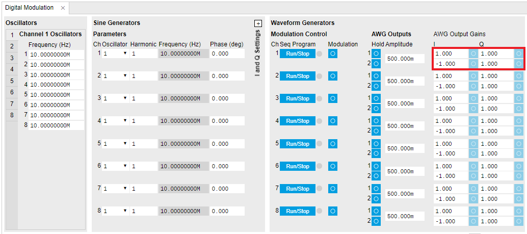
We now look at how the Signal Generator channel of the SHFQC+ actually generates modulated signals. In the LabOne UI, there are four AWG output gains that can be used to set up single-sideband modulation. These AWG output gains are multiplied by the AWG outputs. The AWG output gains can be set individually to make it easier to calibrate DRAG pulses, for example.

Figure 2: Digital Modulation tab in the LabOne UI

When modulation is enabled, the AWG output gains control of the signs and amplitudes of the sinusoids that are multiplied with the AWG outputs. To make use of the four AWG output gains settings needed for a complex, dual-channel signal, the sequencer code must make use of the playWave command in the form playWave(1,2, wI, 1,2, wQ). Figure 3 shows how the different parts of the playWave command map to the different gain nodes in the digital modulation process.

Figure 3: Diagram of digital modulation processing chain and settings. Bolded parts of the text show how the different parts of the 'playWave' command map to the different gain nodes.

We can summarize the signal generated by the FPGA using the following expression:

\[ \begin{equation}\tag{3} \begin{aligned} V_{\mathrm{RF}}(t) = V_0 \, A \, \left[ \mathrm{Gain00} \times w_I (t) \cos (2 \pi f_{\mathrm{Osc}} t + \phi) + \mathrm{Gain01} \times w_Q (t) \sin (2 \pi f_{\mathrm{Osc}} t + \phi) \right] \cos (2 \pi f_{\mathrm{RF}} t) \newline\\ - \left[\mathrm{Gain10} \times w_I (t) \sin (2 \pi f_{\mathrm{Osc}} t + \phi) + \mathrm{Gain11} \times w_Q (t) \cos (2 \pi f_{\mathrm{Osc}} t + \phi) \right] \sin (2 \pi f_{\mathrm{RF}} t) \end{aligned} \end{equation} \]

where \(\mathrm{Gain}ij\) of Channel n corresponds to the node path <dev>/SGCHANNELS/<chan>/AWG/OUTPUTS/<i>/GAINS/<j>. The choice of \(\mathrm{Gain00} = \mathrm{Gain10} = \mathrm{Gain11} = 1.0\) and \(\mathrm{Gain01} = -1.0\) yields the same expression as in Equation 2 and therefore leads to single sideband modulation at the upper sideband for positive oscillator frequencies. Note that in this simplified overview of the digital modulation and upconversion chain, we have lumped together the digital upconversion to 2.0 GHz and the digital-to-analog conversion with the analog upconversion pathway into a single upconversion step. See also In/Out Tab.

Note

Depending on the selected value of \(f_{\mathrm{Osc}}\), the voltage measured on a scope may not correspond exactly to the formula above due to the effect of the filters used in the analog upconversion.

Note

For HDAWG users: The SHFQC+ and HDAWG use different sign conventions for achieving upper sideband modulation. Because the HDAWG is typically used in combination with physical IQ mixers when generating an RF signal, the HDAWG assumes a negative time dependence in the exponential, whereas the SHFQC+ assumes a positive time dependence. To achieve upper sideband modulation on both instruments, there is therefore a relative sign swap needed on the gain settings \(\mathrm{Gain01}\) and \(\mathrm{Gain10}\).

The following table summarizes the parameter names and their corresponding node paths. For more information on setting node values via API, see the Using the Python API Tutorial. See also Node Documentation.

Table 1: Summary of parameters used in AWG signal generation

Parameter name	Symbol	Node path
I waveform	\(w_I (t)\)	Defined in sequence
Q waveform	\(w_Q (t)\)	Defined in sequence
AWG output gains	\(\mathrm{Gain}ij\)	<dev>/SGCHANNELS/<chan>/AWG/OUTPUTS/<i>/GAINS/<j>
Global amplitude	\(A\)	<dev>/SGCHANNELS/<chan>/AWG/OUTPUTAMPLITUDE
Oscillator frequency	\(f_{\mathrm{OSC}}\)	<dev>/SGCHANNELS/<chan>/OSCS/<OSC>/FREQ
Sine generator phase	\(\phi\)	<dev>/SGCHANNELS/<chan>/SINES/0/PHASESHIFT
RF center frequency	\(f_{\mathrm{RF}}\)	<dev>/SYNTHESIZERS/<synth>/CENTERFREQ
Output range	\(P_{\mathrm{max}}\)	<dev>/SGCHANNELS/<chan>/OUTPUT/RANGE

We now show how to generate a modulated AWG signal. We monitor the AWG signal using one channel of an external scope and use the second scope channel for triggering purposes. The following tables summarize the settings to enable the SHFQC+ outputs and configure the sine generator, as well as to configure the external scope.

Table 2: Settings: enable the output

Tab	Section	Sub-Section	Label	Setting / Value / State
In/Out	SG Channel 1		On	ON
In/Out	SG Channel 1		Range (dBm)	10
In/Out	SG Channel 1		Center Freq (Hz)	1.0 G
In/Out	SG Channel 1		Output Path	RF

| Digital Modulation | Waveform Generators | Modulation | 1 | ON | | Digital Modulation | AWG Outputs | Amplitude | | 0.5 | | Digital Modulation | AWG Output Gains | I | 1 | 1.0 | | Digital Modulation | AWG Output Gains | I | 2 | -1.0 | | Digital Modulation | AWG Output Gains | Q | 1 | 1.0 | | Digital Modulation | AWG Output Gains | Q | 2 | 1.0 | | Digital Modulation | Channel 1 Oscillators | Frequency (Hz) | 1 | 10.0 M | | Digital Modulation | Sine Generators | I | En | OFF | | Digital Modulation | Sine Generators | Q | En | OFF | | DIO | Marker | Source | 1 | Output 1 Marker 1 |

Table 3: Settings: Configure the external scope

Scope Setting	Value / State
Ch1 enable	ON
Ch1 range	0.2 V/div
Ch2 enable	ON
Ch2 range	0.5 V/div
Timebase	1 us/div
Trigger source	Ch2
Trigger level	200 mV
Run / Stop	ON

Note

For HDAWG users: Enabling digital modulation on the SHFQC+ is analogous to enabling Sine12 modulation on Wave 1 and Sine21 modulation on Wave 2.

A sine generator is a direct digital synthesis (DDS) unit that converts a digital oscillator signal (essentially just an incrementing phase) to a sinusoid with a certain phase offset and harmonic multiplier using a look-up table containing one period of the sinusoid signal. The digital oscillator in turn is a phase accumulator with a very precise frequency derived from the instrument’s main clock. The digital oscillators on the instrument are represented in the Oscillators section of the Digital Modulation tab. Each Signal Generator output channel of the SHFQC+ has 8 oscillators associated with it, although only one can be used by the sine generator at a time. For details on how to switch between oscillators during a sequence, see the Command Table Tutorial.

In this example, we use a Gaussian pulse for the I waveform and a derivative of a Gaussian for the Q waveform. When combined, this generates a DRAG pulse.

wave w_gauss = gauss(1024, 512, 128);
wave w_drag  = drag(1024, 512, 128);
wave m_high = marker(512, 1);
wave m_low = marker(512, 0);
wave m = join(m_high, m_low);
wave w_gauss_marker = w_gauss + m;

resetOscPhase();

playWave(1,2, w_gauss_marker, 1,2, w_drag);

We also configure the FFT settings on the scope.

Table 4: Settings: Configure the external scope

Scope Setting	Value / State
Acquisition Time	10 us
FFT Center	1 GHz
FFT Span	100 MHz
Resolution BW	200 kHz

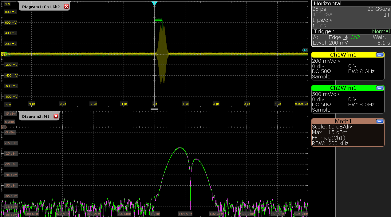
Save and play the Sequencer program with the above settings. The upper plot in Figure 4 shows the AWG signals captured by the scope. We see that the resulting DRAG pulse is a combination of a Gaussian waveform with a derivative of a Gaussian waveform generated by the drag() function in SeqC. The FFT of the scope trace shows that there is a dip in the spectrum, a key characteristic of the DRAG pulse combination.

Figure 4: Dual-channel signal generated by the AWG and captured by the scope. The top half of the figure shows a pulse that is a combination of a Gaussian pulse and a derivative of a Gaussian pulse, modulated at 10 MHz and upconverted with an RF center frequency of 1.0 GHz. The bottom part of the figure shows the FFT of the scope trace, demonstrating the characteristic spectral dip of the DRAG pulse.

Note

There are two ways of generating AWG signals with a single frequency component at the front panel output when digital modulation is enabled. For completely real signals that require only a single AWG output, playWave(1,2, wI) suffices to generate a single sideband signal. For complex signals requiring dual-channel waveforms, playWave(1,2, wI, 1,2, wQ) is needed.

Note

To avoid saturating the output when using playWave(1,2, wI, 1,2, wQ) syntax, it is necessary to either set the value of the global amplitude to 0.5 or to scale the waveform in the sequencer code similarly. A value of up to 1.0 can safely be used when playWave(1,2, wI) is used for generating single sideband real signals.

So far in this tutorial, we have shown how to achieve single sideband modulation with the playWave command, but to efficiently use the instruction memory of the SHFQC+ and ensure smooth, back-to-back waveform playback, it is recommended to use the command table, which requires assigning the waveform an index and using the executeTableEntry command instead of playWave. To assign an index of 0 to a waveform, the command assignWaveIndex(1,2, wI, 0) should be used for single-AWG-channel signals and assignWaveIndex(1,2, wI, 1,2, wQ, 0) for dual-channel signals. For more details, see the Command Table Tutorial.

Rapid Phase Changes

The SHFQC+ supports rapid, real-time changes of the carrier phase in modulation mode through the sequencer instructions setSinePhase and incrementSinePhase, as well as through the command table. This capability is particularly valuable when generating long patterns of pulses with varying phases, e.g. to account for AC Stark shift in qubit control sequences, or to realize phase cycling protocols.

In addition, there is the possibility to reset the starting phase of one or multiple oscillators at the beginning of a pulse sequence using the resetOscPhase instruction. Thus it can be ensured that the carrier-envelope offset, and thus the final output signal, is identical from one repetition to the next.

In the following AWG sequencer program, we generate a series of 4 dual-channel square pulses that are played back-to-back. We initialize the oscillator phase by a resetOscPhase instruction. In this form without an argument, the instruction will reset the phases of all oscillators accessible by this core (here oscillators 1 through 8 of Channel 1). Alternatively, an argument in binary representation, e.g. 0b0101, allows us to reset only a subset of these oscillators. We then set the phase of the sine generator to 45 degrees using the setSinePhase instruction. Subsequently, we play back the dual-channel waveform 4 times, and after each playback instruction, we increase the phase of the sine generator by 90 degrees. The corresponding instruction incrementSinePhase takes effect at the end of the previous waveform playback, which allows us to change the phase precisely in between waveforms. Upload the following sequence program to the AWG and run the sequence.

const LENGTH = 48;

wave w = ones(LENGTH);
wave m_high = marker(LENGTH/2, 1); //marker high
wave m_low = marker(LENGTH/2, 0); //marker low
wave m = join(m_high, m_low); //join marker waveforms
wave wm = w + m; //combine marker and ones waveform data

while (true) {
    resetOscPhase();

    setSinePhase(45);
    playWave(1,2, wm);

    incrementSinePhase(90);
    playWave(1,2, w);

    incrementSinePhase(90);
    playWave(1,2, w);

    incrementSinePhase(90);
    playWave(1,2, w);
}

Configure the scope according to the following settings.

Table 5: Settings: Configure the external scope

Scope Setting	Value / State
Ch1 enable	ON
Ch1 range	0.2 V/div
Ch2 enable	ON
Ch2 range	0.5 V/div
Timebase	10 ns/div
Trigger source	Ch2
Trigger level	200 mV
Run / Stop	ON

We also change the oscillator frequency to make it easier to visual the phase changes.

Table 6: Settings: enable the output

Tab	Section	Sub-Section	Label	Setting / Value / State
Digital Modulation	Channel 1 Oscillators	Frequency (Hz)	1	-500.0 M

Figure 5 shows the resulting signal. Three of the instantaneous phase increments of 90 degrees are visible as transient features. In a real use case, the phase changes usually occur in between pulses when the envelope signal is zero-valued, and these transients are then absent.

Figure 5: Amplitude-modulated dual-channel signal with rapid real-time phase increments generated by the SHFQC+.

Note

The phase increment due to the incrementSinePhase instruction takes effect at the end of the previous waveform playback. In case the instruction is placed in the sequencer code before the first playWave instruction, the phase increment will only happen after the playWave instruction.

Performing Frequency Sweeps

By using the sequencer commands setOscFreq, configFreqSweep, and setSweepStep, it is possible to set the oscillator frequency as part of a sequence and even perform frequency sweeps quickly while using a minimum number of sequencer instructions. Using these instructions, the oscillator frequency can be changed on a timescale of approximately 100 ns. The timing of the frequency update is deterministic. The waveforms that follow the frequency update will wait until the update has finished. A waitWave command after the waveform playback instructions is required to ensure that any subsequent frequency update does not happen during the waveform playback.

Note

The setOscFreq, configFreqSweep, and setSweepStep commands are intended to change the oscillator frequency between pulses. To sweep the frequency during a pulse, it’s best to encode the frequency change in the waveform, e.g. using the chirp waveform generation function.

const START_FREQ = -100e6; //start frequency in Hz
const FREQ_INC = 200; //increment in Hz
const N_STEPS = 1e6; //number of frequency steps
const OSC = 0; //oscillator to sweep

const MEAS = 2048; //measurement window in samples

const LENGTH = 160; //length of pulse in samples

wave w = gauss(LENGTH, 1, LENGTH/2, LENGTH/8);
wave m_high = marker(LENGTH/2, 1); //marker high
wave m_low = marker(LENGTH/2, 0); //marker low
wave m = join(m_high, m_low); //join marker waveforms
wave wm = w + m; //combine marker and ones waveform data

//set up frequency sweep
configFreqSweep(OSC,START_FREQ,FREQ_INC);

var i;
for (i = 0; i < N_STEPS; i++) {
  setSweepStep(OSC,i);

  resetOscPhase();

  playWave(1,2, wm);
  playZero(MEAS);
  waitWave(); //to ensure setSweepStep does not execute during the play instructions
}

Upload and run the above sequencer code on the AWG core of the Signal Generator channel 1. To make it easier to observe the frequency sweep on a scope, the length of the MEAS constant can be increased (e.g. with a measurement length of 2e8 samples, the frequency will update every 10 ms).

Note

Multiple frequency sweeps can be configured in parallel, such that each oscillator of a given channel can be swept independently of the others.