Continuous Resonator Spectroscopy
Note
This tutorial is applicable to all SHFQC+ Instruments.
Goals and Requirements
The goal of this tutorial is to demonstrate how to use the SHFQC+ to perform resonator spectroscopy measurement using the Quantum Analyzer readout channel with the LabOne User Interface (UI) and Zurich Instruments Toolkit API.
Note
For zhinst-toolkit users, please find the example in https://github.com/zhinst/zhinst-toolkit/blob/main/examples/shfqc_resonator_spectroscopy_cw.md , and the zhinst-toolkit documentation.
For LabOne Q users, please find the example in https://github.com/zhinst/laboneq/blob/main/examples/01_qubit_characterization/01_cw_resonator_spec_shfsg_shfqa_shfqc.ipynb and https://github.com/zhinst/laboneq/blob/main/examples/01_qubit_characterization/02_pulsed_resonator_spec_shfsg_shfqa_shfqc.ipynb, and the LabOne Q User Manual.
Preparation
Please follow the preparation steps in Connecting to the Instrument and connect the instrument in a loopback configuration as shown in Figure 1 or to a device under test.

Tutorial
In this tutorial, we sweep frequency of output signal and measure the frequency response of the cable or the device under test.
This section shows how to use the LabOne UI to configure the instrument, run the measurement and monitor the measurement results.
-
Configure the instrument
-
Set center frequency and power range of input and output signals
Configure these parameters on the Input and Output Tab as in Figure 2 and in Table 1.
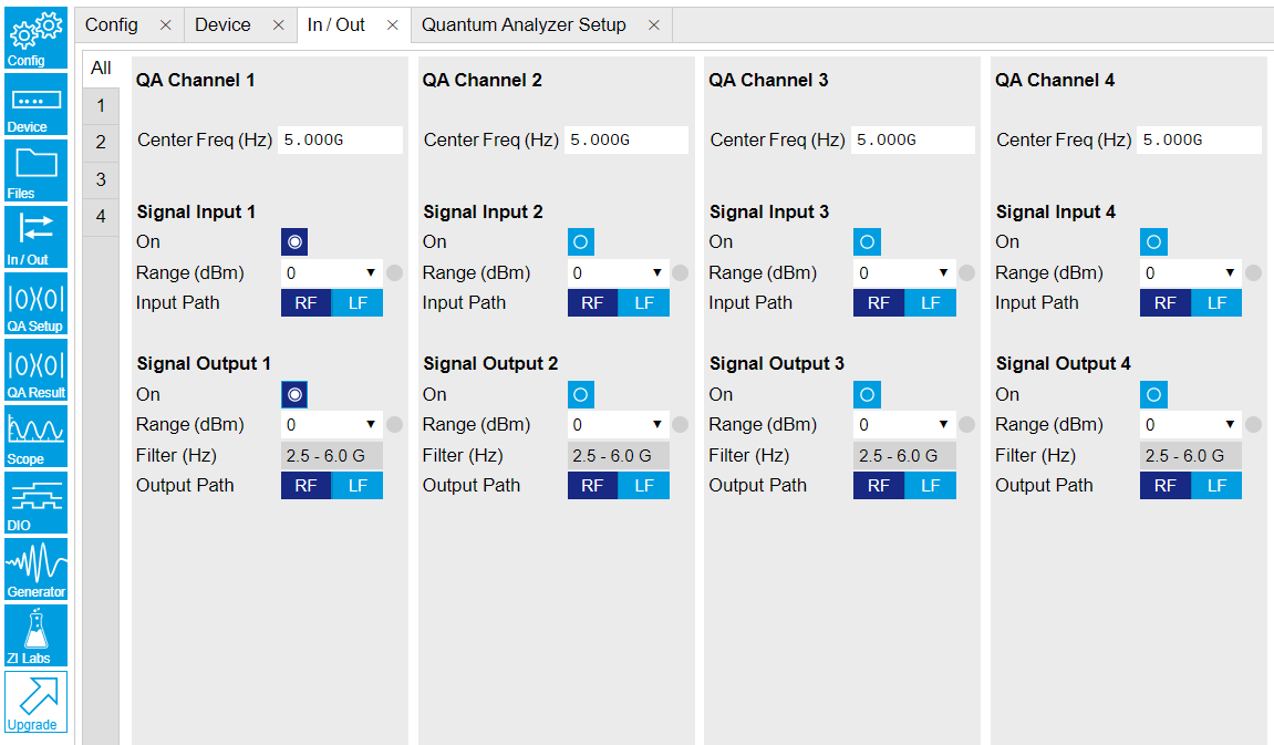
Figure 2: Configurations on In/Out Tab. Table 1: Settings of QA Channel 1 on In/Out Tab Parameter Setting Description QA Channel Selection All Select All to display all QA Channels. Cent Freq (Hz) 5 GHz Set center frequency of the frequency sweep. Signal Input 1 On Enable Enable the Signal Input 1. Signal Input 1 Range (dBm) 0 dBm Set power range of Signal Input 1 to 0 dBm. This setting allows the instrument to acquire a input signal with a power up to 0 dBm. Signal Input 1 Input Path RF Set input path of Signal Input 1 to RF path. Signal Output 1 On Enable Enable the Signal Output 1. Signal Output 1 Range 0 dBm Set power range of Signal Output 1 to 0 dBm. This setting allows the instrument to output a signal with a power up to 0 dBm. Signal Output 1 Output Path RF Set output path of the Signal Output 1 to RF path. -
Upload and compile measurement sequence
The measurement sequence is defined on the Sequence sub-tab of the Readout Pulse Generator tab, see Figure 3 and Table 2.
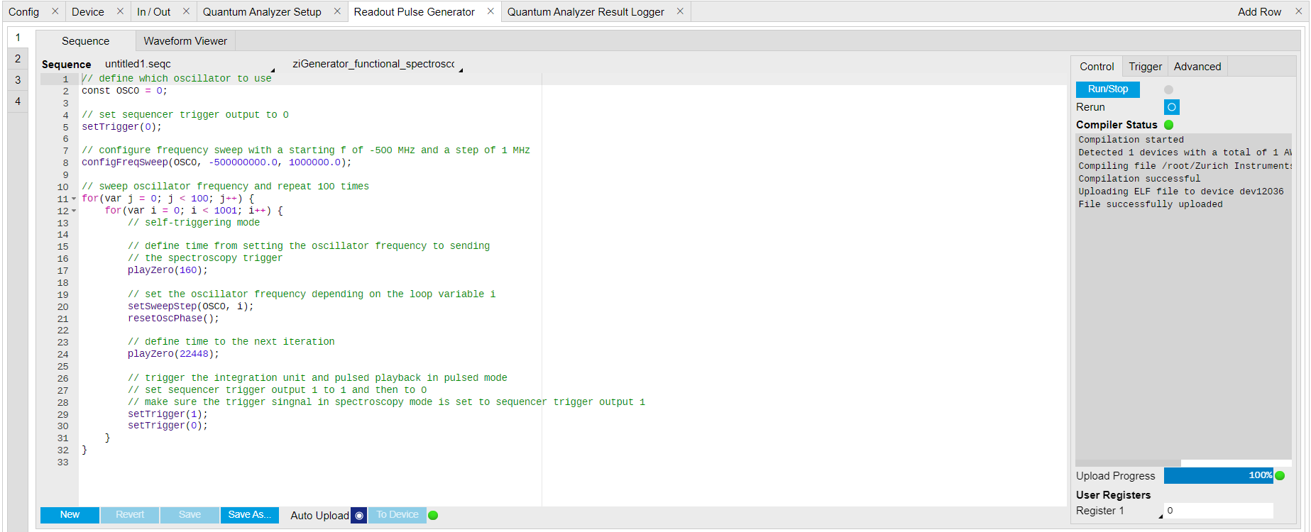
Figure 3: Configurations on Readout Pulse Generator Tab. Table 2: Settings of QA Channel 1 on Readout Pulse Generator Tab. Parameter Setting Description QA Channel Selection 1 Select QA Channel 1. Sub-Tab Display Sequence Select Sequence sub-tab and paste the sequence program below or load ziGenerator_functional_spectroscopy.seqc from the "Examples" library and modify it. The Waveform Viewer sub-tab displays readout envelope if it is uploaded. Compile Click "To Device" Compile the sequence program by clicking "To Device". Return Disable Disable return function. Run/Stop Disable Disable Run/Stop. Below is the the sequence program for the measurement. In the inner loop, the
setSweepStep(OSC0, i)command sets frequency of digital oscillator 0 to i-th frequency in an array configured byconfigFreqSweep(OSC0, -500000000.0, 1000000.0)command, thesetTrigger(value)command sets Sequencer Trigger 1 Output to high and then low to start integration, and waveform generation if pulsed waveform is desired, theplayZero(samples)command define time to the nextplayZero(samples). The measurement is repeated 100 times by the outer loop.// define which oscillator to use const OSC0 = 0; // set sequencer trigger output to 0 setTrigger(0); // configure frequency sweep with a starting f of -500 MHz and a step of 1 MHz configFreqSweep(OSC0, -500000000.0, 1000000.0); // sweep oscillator frequency and repeat 100 times for(var j = 0; j < 100; j++) { for(var i = 0; i < 1001; i++) { // self-triggering mode // define time from setting the oscillator frequency to sending // the spectroscopy trigger playZero(160); // set the oscillator frequency depending on the loop variable i setSweepStep(OSC0, i); resetOscPhase(); // define time to the next iteration playZero(22448); // trigger the integration unit and pulsed playback in pulsed mode // set Sequencer Trigger Output 1 to high and then to low // make sure the trigger singnal in spectroscopy mode is set to sequencer trigger output 1 setTrigger(1); setTrigger(0); } } -
Configure signal generation and data acquisition
Signal generation and data acquisition are defined on QA Setup Tab and QA Result logger Tab. The baseband readout signal is generated by a digital oscillator directly ("Continuous"), or by mixing the signal from the digital oscillator and a waveform envelop saved in the waveform memory ("Pulse"). The input signal after frequency down-conversion is integrated for 512 ns started 224 ns later after receiving a trigger from Sequencer 1 Trigger Output 1.
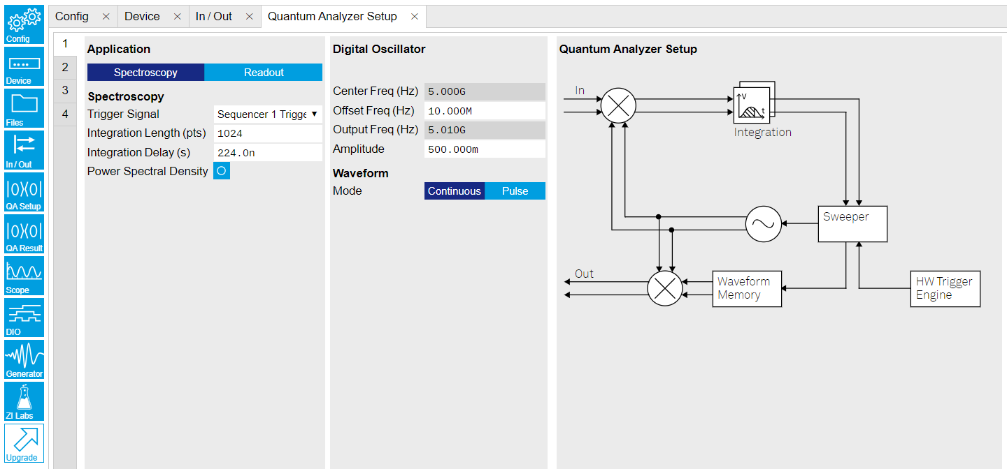
Figure 4: Configurations on QA Setup Tab. Table 3: Settings of QA Channel 1 on QA Setup Tab, see details on Parameter Setting Description QA Channel Selection 1 Select QA Channel 1. Application Mode Spectroscopy Use spectroscopy mode for resonator spectroscopy measurement. In spectroscopy mode, frequency sweep is done by sweeping the frequency of the digital oscillator. Trigger Signal Sequencer 1 Trigger Output 1 Select Sequencer 1 Trigger Output 1 as the trigger source to trigger both output pulse generation and integration. This selection matches the trigger setting written in the sequence program. Integration Length (pts) 1048 Set the integration length in number of samples. Integration Delay (s) 224n Set the delay time after receiving a trigger before starting integration. This setting ensures only expected input signal is integrated. The internal delay from signal generation to integration is about 224 ns. Therefore integration delay is > 224 ns if the propagation delay from front panel signal output port to signal input port is not negligible. Power Spectral Density Disable Disable the Power Spectral Density measurement function. Digital Oscillator Amplitude 0.5 Set the amplitude factor of the digital oscillator to 0.5. The range of amplitude factor is from 0 to 1. Waveform Mode Continuous Set the Waveform Mode to continuous, so the output waveform is continuous. Select "Pulse" and upload a .csv file with complex data for waveform envelope if pulsed output waveform is desired. On the QA Result Logger Tab, it defines the source of the result, and how the result is averaged and displayed, see Figure 5 and Table 4. After configuration of all parameters, the QA Result Logger should be enabled to be ready to receive measurement results.
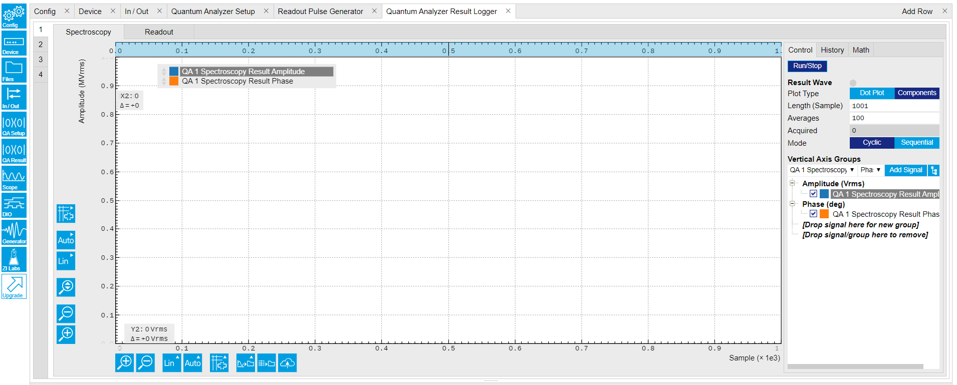
Figure 5: Configurations on QA Result Logger Tab. Table 4: Settings of QA Channel 1 on QA Result Logger Tab. Parameter Setting Description QA Channel Selection 1 Select QA Channel 1. Sub-Tab Spectroscopy Select Spectroscopy sub-tab to monitor measurement result when using the Spectroscopy mode. Plot Type Components Select Components to display I, Q, amplitude or phase versus sample points. Select Dot Plot to display I versus Q with scattered dots. Result Length (Sample) 1001 Set result length in number of samples. The number must match what is set in the sequence program. Averages 100 Set number of averages. The number must match what is set in the sequence program. Average Mode Cyclic Set the average mode to cyclic. This setting must match how the loop is configured in the sequence program. Vertical Axis Groups Add amplitude and phase Select amplitude and phase to be displayed on the plot. Run/Stop Enable Enable the result logger to receive and display measurement results.
-
-
Run the measurement
By clicking "Run/Stop" icon on the Readout Pulse Generation Tab, the measurement is started and finished in seconds.
-
Monitor the measurement result
The measurement result (complex data) is normalized by the integration length and displayed on the QA Result Tab, as shown in Figure 6. Select "Dot Plot" to display result in IQ (complex) plane.
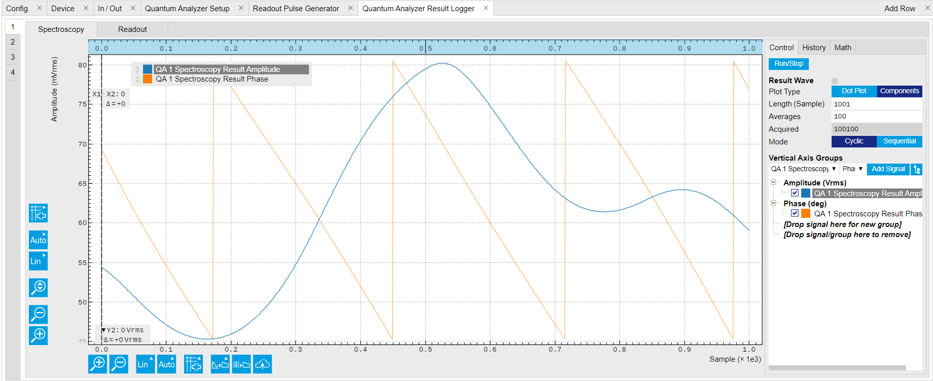
Figure 6: Measurement results on the QA Result Logger Tab.
In specific, we demonstrate how to run a frequency sweep, obtain the transmission data and plot it. For this, the Sweeper is configured to enable a continuous output signal that first probes the device under test and is then correlated with the generated signal. As a result, we obtain the amplitude and phase response in transmission of our device under test.
-
Connect the Instrument
Create a toolkit session to the data server and connect the Instrument with the device ID, e.g. 'DEV12001', see Connecting to the Instrument.
# Load the LabOne API and other necessary packages from zhinst.toolkit import Session DEVICE_ID = 'DEVXXXXX' SERVER_HOST = 'localhost' session = Session(SERVER_HOST) ## connect to data server device = session.connect_device(DEVICE_ID) ## connect to device -
Create a Sweeper and configure it
Python API SHFSweeper class is the core of the spectroscopy measurements. It defines all relevant parameters for frequency sweeping and sequencing. Toolkit wraps around the SHFSweeper and exposes an interface that is similar to the LabOne modules, meaning the parameters are exposed in a node tree like structure.
sweeper = session.modules.shfqa_sweeper
sweeper.device(device)
CHANNEL_INDEX = 0 # physical Channel 1

sweeper.sweep.start_freq(-500e6) # in units of Hz
sweeper.sweep.stop_freq(500e6) # in units of Hz
sweeper.sweep.num_points(1001)
sweeper.sweep.oscillator_gain(0.8) # amplitude scaling factor, 0 to 1
sweeper.sweep.use_sequencer = True # True (recommended): sequencer-based sweep; False: host-driven sweep

sweeper.average.integration_delay(224e-9) # internal delay is about 224 ns
sweeper.average.integration_time(10e-6) # in units of second
sweeper.sweep.wait_after_integration(1e-6) # waiting 1 us after integration before starting a new measurement
sweeper.average.num_averages(200)
sweeper.average.mode("sequential") # "sequential" or "cyclic" averaging

sweeper.rf.channel(CHANNEL_INDEX)
sweeper.rf.center_freq(5e9) # in units of Hz
sweeper.rf.input_range(0) # in units of dBm
sweeper.rf.output_range(0) # in units of dBm

with device.set_transaction():
    device.qachannels[CHANNEL_INDEX].input.on(1)
    device.qachannels[CHANNEL_INDEX].output.on(1)
All available settings of the Sweeper can be find using this command.
list(sweeper)The data class RfConfig includes the channel-specific settings, such as the center frequency in units of Hz, and the power ranges of the Input and Output channel.
The data class SweepConfig allows to configure the sweeps start and stop frequency as the in-band offset frequency. In addition, it contains the number of measured points in the sweep 'num_points', and the mapping of the points ('linear' or 'logarithmic'). The gain of the oscillator 'oscillator_gain' changes the output amplitude of the probe signal relative to the channels power ranges. Hence, the output power of the probe signal hence changes quadratically with this number.
Please note that in this example, the configuration option
use_sequenceris not explicitly set to its default valueTrue. In this mode, a SeqC program is automatically generated, uploaded and compiled in the SHFQC+ Sequencer, and the frequency of the digital oscillator is controlled by the Sequencer. This mode allows a fast resonator spectroscopy with predicted cycle time of \(t_{\mathrm{settling\ time}} + t_{\mathrm{integration\ delay}} + t_{\mathrm{integration\ time}} + t_{\mathrm{wait\ after\ integration}}\), see Table 5. Ifset_sequencerisFalse, the sweeper is controlled by the host computer, and the frequency sweep is slower.The data class AvgConfig contains all settings related to averaging and integration. The 'integration_time' defines how long the signal is integrated in the qubit_measurement_unit, which can be up to \~16.7 ms. The mode 'sequential' or 'cyclic' define, whether each point is first averaged 'num_averages' times before the frequency is changed, or whether every sweep is averaged 'num_averages' times.
Please note that default values of Sweeper parameters listed in Table 5 depend on the
zhinstversion.Table 5: Default values of Sweeper parameters. Parameter Description Default Value for zhinst < 22.08 Default Value for zhinst >= 23.02 settling time Waiting time after having set the new frequency until issuing the setTriggercommand, which triggers the spectroscopy unit.200 ns 80 ns integration delay Delay after the internal trigger arrives at the spectroscopy unit until the integration of the input signal starts. 0 ns 224 ns
(zhinst-utils version ≥ 0.1.5)envelope delay Delay After the internal trigger arrives at the spectroscopy unit until the playback of the envelope waveform starts. 0 ns 0 ns integration time Time to integrate the input data. 1 ms 1 ms wait after integration Wait time after the end of the integration until the start of the next cycle. 72 ns 0 ns predicted cycle time Calculated duration of each cycle of the spectroscopy loop. Note that this property only applies in self-triggered mode, which is active when the trigger source is set to Noneanduse_sequencerisTrue.- "settling time" + "integration delay" + "integration time" + "wait after integration"
(read-only) -
Run the measurement with continuous output waveform and plot the data
result = sweeper.run()
num_points_result = len(result["vector"])
print(f"Measured at {num_points_result} frequency points.")
sweeper.plot()
After executing
sweeper.run(), all above parameters are updated, and a SeqC program is automatically generated, uploaded and compiled based on the sweep parameters, see in Figure 7. In the program,ConfigFreqSweepsets the start frequency and the frequency increment in units of Hz for a chosen oscillator, andsetSweepStepsets the oscillator frequency. The oscillator phase is reset byresetOscPhasebefore each measurement. The trigger generated in the sequencer is used to start the integration, and theplayZerosets the cycle duration. The measurement is repeated using the nestedforloop according to the averaging mode. The measurement starts after enabling the sequencer.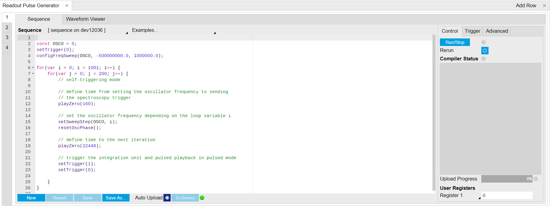
Figure 7: Seqc program in the Readout Pulse Generator Tab. The result returned from
sweeper.run()is complex data \(E_{\mathrm{sweeper}}\) in units of Vrms. It is averaged and normalized by the integration length. The power \(P\) and phase \(\phi\) can be calculated as,\[ \begin{equation}\tag{1} \begin{aligned} P & = 10\lg(\frac{|E_{\mathrm{sweeper}}|^2}{R}1000), \newline \phi & = \arctan\frac{\Im(E_{\mathrm{sweeper}})}{\Re(E_{\mathrm{sweeper}})}, \end{aligned} \end{equation} \]where \(R\) is 50 \(\Omega\), 1000 is the conversion factor from W to mW. With
sweeper.plot(), the power and phase are calculated and plotted, see Figure 8.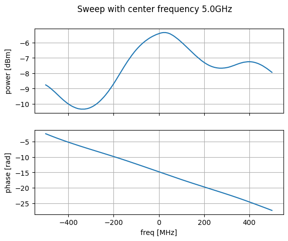
Figure 8: Measurement result with continuous waveform output. -
Run the measurement with pulsed output waveform and plot the data
In contrast to continuous readout waveform generation, pulsed readout waveform generation requires an envelope data. Create a complex flat-top Gaussian envelope with 10 μs duration and 50 ns rise and fall time. Enable the pulsed mode by
sweeper.envelope.enable(True)and upload the envelope to the waveform memory. This envelope can be displayed on the Waveform Viewer of the Readout Pulse Generator.from scipy.signal import gaussian import numpy as np SAMPLING_FREQUENCY = 2e9 # in units of Hz ENVELOPE_DURATION = 10.0e-6 # in units of second ENVELOPE_RISE_FALL_TIME = 0.05e-6 # in units of second rise_fall_len = int(ENVELOPE_RISE_FALL_TIME * SAMPLING_FREQUENCY) std_dev = rise_fall_len // 10 gauss = gaussian(2 * rise_fall_len, std_dev) complex_amplitude = (1 - 1j)/np.sqrt(2) flat_top_gaussian = np.ones(int(ENVELOPE_DURATION * SAMPLING_FREQUENCY)) * complex_amplitude flat_top_gaussian[0:rise_fall_len] = gauss[0:rise_fall_len] * complex_amplitude flat_top_gaussian[-rise_fall_len:] = gauss[-rise_fall_len:] * complex_amplitude sweeper.average.integration_delay(224e-9) # in units of second sweeper.envelope.enable(True) # True: Pulsed mode; False: Continuous mode sweeper.envelope.waveform(flat_top_gaussian) # upload envelope waveform result = sweeper.run() num_points_result = len(result["vector"]) print(f"Measured at {num_points_result} frequency points.") sweeper.plot()After executing
sweeper.run(), all above parameters are updated, a SeqC program is automatically generated, uploaded and compiled based on the sweep parameters, see Figure 7, and the result is downloaded after the measurement is done. The power and phase are calculated, see in Figure 9. The result is consistent with measurement with continuous waveform output.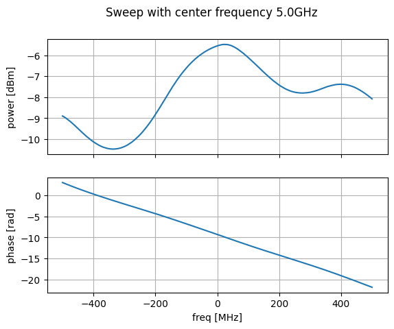
Figure 9: Measurement results with pulsed waveform output.