Basic Qubit Characterization

Note

This tutorial is applicable to all HDAWG Instruments.

Goals and Requirements

In this tutorial, we demonstrate how to generate pulse sequences for basic quantum bit (qubit) characterization. We develop a basic qubit characterization sequencer program in which we implement pulse sequences to measure a qubit’s lifetime, and demonstrate how to perform Rabi, Ramsey, and spin-locking experiments.

To visualize the generated output signals of the HDAWG, an oscilloscope with sufficient bandwidth and at least 3 channels is required.

Preparation

Make sure that the instrument is powered on and connected by USB to your host computer or by Ethernet to your local area network (LAN) where the host computer resides. After starting LabOne, the default web browser opens with the LabOne graphical user interface.

The tutorial starts with the instrument in the default configuration (e.g., after a power cycle) and the default user interface settings (e.g., as is after pressing F5 in the browser). We will monitor the HDAWG outputs using two channels of an external scope, and use a third scope channel for visualizing a trigger. Connect the HDAWG’s outputs to the oscilloscope as follows:

The following table summarizes the settings used to configure the external scope.

Table 1: Settings: Configure the external scope

Scope Setting	Value / State
Ch1-3 enable	ON
Ch1-2 range	0.2 V/div
Ch3 range	1 V/div
Timebase	5 us/div
Trigger source	Ch3
Trigger level	500 mV
Run / Stop	ON

Qubit Characterization Setup and Measurement Procedure

This tutorial can be directly applied to the circuit QED (cQED) measurement setup shown in Figure 1. This setup contains both the HDAWG and the UHFQA Quantum Analyzer. Note that it can be modified to accommodate other measurement systems or implementations with minimal effort. Here, a qubit control pulse (green) at microwave frequencies is generated with IQ-based upconversion using the signal outputs Wave 1 and 2 of the HDAWG. Upon receiving a trigger pulse (red) generated by the marker output (Mark 1) of the HDAWG, the qubit’s state is then read out (blue) by measuring the signal transmission of the resonator using the UHFQA Quantum Analyzer in combination with IQ-based up-/down conversion to/from the microwave regime.

Figure 1: Experimental measurement setup and visualization of key signals. The element labeled as Q

IQ-based up-conversion: An IQ-mixer generates a single amplitude- and phase-controlled signal at frequency f_LO-f_IF from two directly synthesized I and Q quadrature signals at intermediate frequency f_IF and a local oscillator at frequency f_LO. The otherwise identical I and Q signals only differ in their relative amplitude and phase of approximately -90° that need to be calibrated to suppress spurious signals.

Resonator readout: A qubit that is dispersively coupled to a resonator shifts the resonator’s frequency depending on whether it is in its ground (|g>) or excited (|e>) state. Upon receiving a rising-edge trigger from the HDAWG at Trigger 1, the UHFQA detects this shift and determines the state of the qubit by measuring the change in amplitude and/or phase of a microwave pulse probing the resonator’s transmission at a specific frequency f_Res, as indicated by the double arrow in the inset of the Figure.

Measurement Setup Variations for other Qubit Platforms

Different physical platforms such as cQED, spin qubits, ions, or atoms have varying requirements for their setups. In this tutorial, we will refer to the following variations to highlight small changes to the workflow: - Variation 1: Qubit control pulse (atoms/ions). In an atom/ion platform, single-qubit manipulation is often performed by controlling the intensity of a laser with an acousto-optic modulator. In this case, a single channel of the HDAWG is sufficient to directly synthesize a control pulse at the required carrier frequency (typically between 80 MHz and 200 MHz). The phase-sensitive applications of the tutorial may no longer pertain unless a dedicated system enables phase control of the qubit-addressing lasers. - Variation 2: Square-shaped readout pulse (cQED). In the absence of a dedicated readout-pulse synthesizer, a square pulse is often generated using a microwave switch and a TTL-compatible trigger signal. The Marker output (Mark) of the HDAWG is able to generate a suitable signal that controls the length of the readout pulse.

Generic Sequence Structure

In this part we discuss a generic qubit characterization sequencer program and the HDAWG setup required for this task. The goal is to generate a simple qubit control pulse using this program. All other qubit characterizations discussed in this tutorial will use the same structure and setup.

When programming qubit control sequences with the HDAWG, it is advisable to only program pulse envelopes, and use the integrated oscillators and sine generators that come with every HDAWG to generate the carrier signals needed for IQ-based up-conversion (Digital Modulation). This approach has two advantages. First, it avoids the explicit programming of pulse modulations in the sequencer program sample by sample. Second, it is directly scalable for frequency-multiplexed multi-qubit control. Note that the phase control of the sine generators is a useful tool for qubit control, e.g. it can be used to apply single-qubit gates along every axis of the Bloch sphere. The following table summarizes the settings for the HDAWG Wave outputs.

Table 2: Settings: enable the HDAWG outputs and oscillator control

Tab	Sub-tab	Section	#	Label	Setting / Value / State
Output		Oscillators	1	Frequency (Hz)	10 MHz
Output		Oscillators		AWG Oscillator Control	ON
Output		Waveform Generators	1	Modulation	Sine 11
Output		Waveform Generators	2	Modulation	Sine 22
Output		Wave Outputs	1	Range	0.8 V
Output		Wave Outputs	2	Range	0.8 V
Output		Wave Outputs	1	Enable	ON
Output		Wave Outputs	2	Enable	ON

Note

Depending on the experimental setup, the oscillator frequency (f_IF) should be set such that the final pulse frequency f_LO-f_IF is resonant with the qubit frequency.

Variation 1: The recommended value for f_IF is the center frequency of the acousto-optic modulator.

Note

The AWG Oscillator Control button can only be enabled if the oscillators are correctly matched to the sine generators, e.g. as given by the standard settings.

Note

Depending on the experimental setup, e.g. the insertion loss of the IQ-mixer in use, the 'Range' of Wave Outputs 1 and 2 should be adjusted accordingly.

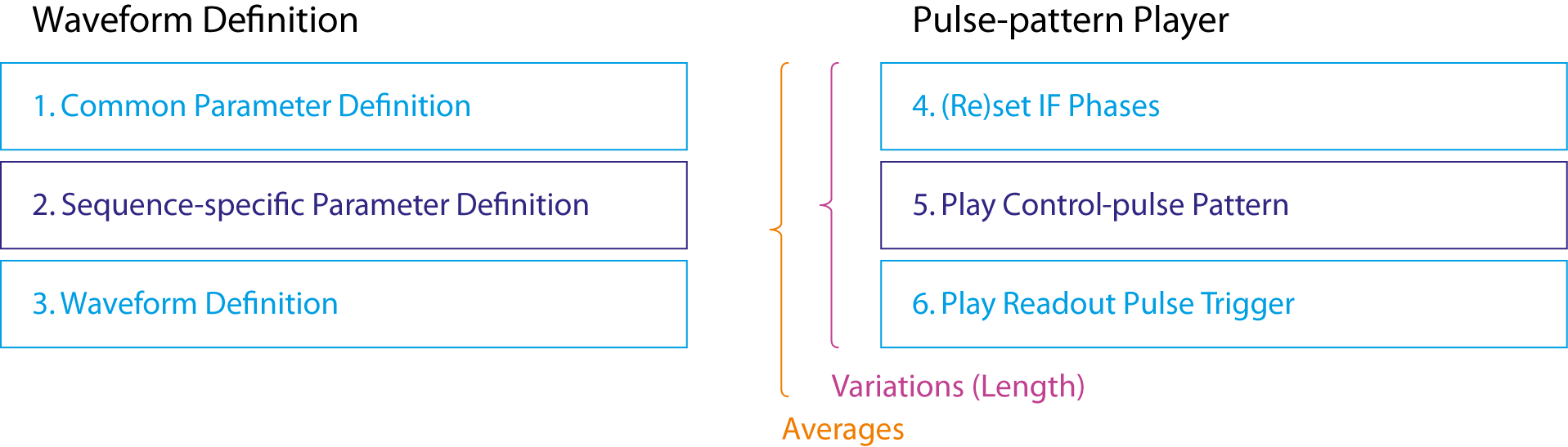
Figure 2 illustrates the generic structure for all sequence programs used in this tutorial. It consists of two parts, the 'waveform definition' and the 'pulse-pattern player'. The segments in light blue (segments 1, 3, 4, 6) are common to all the following examples; only the ones in dark blue (segments 2 and 5) will change.

Figure 2: Structure of the qubit characterization sequencer program

To start, we generate a single qubit control pulse. The following sequencer program implements a Gaussian pulse within the above sequence structure and may be copied into the HDAWG Sequence Editor as is.

//// Waveform definition

//// (1) Common Parameter Definition
// Clock parameters
const sample_clock = 2.4e9;  // Hz
const sequencer_clock = sample_clock/8;  // Hz

// Control-pulse parameters
const pulse_length = 1.9e-6;  // s
const pulse_width = 0.187e-6;  // s
const pi_amp = 1;  // relative to HDAWG output range
const pi2_amp = 0.5;  // relative to HDAWG output range
const rel_iq_amplitude = 0.9;  // relative to programmed pulse height
                               // (dependent on mixer calibration)
const rel_iq_phase = 270;  // deg (dependent on mixer calibration)

// Readout-pulse parameters
const readpulse_time = 12e-9;  // s; account for cable-length mismatch
const readpulse_length = 2e-6;  // s; define trigger length for readout pulse
const qubit_lifetime = 100e-9;  // s

// Convert time to HDAWG samples and round to sequencer resolution
const pulse_length_samples =  round(pulse_length*sample_clock/16)*16;
const pulse_width_samples = round(pulse_width*sample_clock);
const readpulse_time_samples =  round(readpulse_time*sample_clock/16)*16;
const readpulse_length_samples = round(readpulse_length*sample_clock/16)*16;
const qubit_lifetime_samples = round(qubit_lifetime*sequencer_clock);

//// (2) Sequence-specific Parameter Definition
const averages = 1;  // number of repetitions for signal averaging
const length = 1;  // number of parameter variations through experimental sequence

//// (3) Waveform Definition
wave gauss_pulse = gauss(
  pulse_length_samples, 1, pulse_length_samples/2, pulse_width_samples
);

//// Pulse-pattern Player

var j;
for (j = 0; j < averages; j = j + 1) {
  cvar i;
  for (i = 0; i < length; i = i + 1) {
    //// (4) (Re)set IF phases
    resetOscPhase(1);
    setSinePhase(0, rel_iq_phase);
    wait(30);

    //// (5) Play Control-pulse Pattern
    playWave(pi_amp*gauss_pulse, pi_amp*rel_iq_amplitude*gauss_pulse);
    playZero(readpulse_time_samples);

    //// (6) Play Readout Pulse Trigger
    waitWave();
    setTrigger(1);
    playZero(readpulse_length_samples);
    waitWave();
    setTrigger(0);

    wait(5*qubit_lifetime_samples);
  }
}

In segment (1) in waveform definition, we define two clock frequencies, the sample_clock based on which the pulses are synthesized, and the sequencer_clock for instructions from the sequencer. For all qubit characterizations, we use Gaussian pulses of a fixed waveform length (pulse_length) and pulse width (pulse_width) and only vary their pulse amplitudes. The two most important pulse amplitudes, pi_Amp and pi2_Amp, correspond to a π and a π/2-rotation of the qubit, respectively. These can be determined from a Rabi measurement (Rabi Oscillation Measurement). The relative amplitude and phase shift of the two quadratures we generate with the HDAWG and play at the Wave outputs depend on the IQ mixer calibration. We define them using rel_iq_amplitude and rel_iq_phase . With readpulse_time, we can align the start of the readout pulse with the last qubit characterization pulse. This parameter allows us to compensate the difference in delay between the control and readout signal path, e.g. due to different cable lengths. The parameter readpulse_length defines the readout pulse length in Variation 2. We wait for a multiple of the qubit’s lifetime (qubit_lifetime) after the readout pulse before generating the next control pulse in order to let the qubit relax back to its ground state. At the end of segment (1), we convert the parameters expressed in units of time into units of samples or sequencer clock cycles to conform with the main rules for a sequencer program: - All arguments of wait()-functions need to be integers of the sequencer clock cycles (here: 3.3 ns). - All waveform lengths need to be multiples of 16 sample-clock cycles to comply with the waveform granularity specification.

!!! note

  The pulse parameters affecting the shape of a waveform, e.g. the pulse
  width, don’t need to be rounded off even if they are in units of
  samples.

We set the number of different pulse patterns (length) and averages of the experiment (averages) to 1 in segment (2). These correspond to the UHFQA Result Length and Averages settings, respectively. In segment (3), we program a Gaussian pulse with a length of pulse_width and the full-range amplitude.

In the pulse-pattern player part we loop over all different pulse patterns and repeat the full pulse sequence averages times. Note that the sequencer code prohibits the use of a compile-time variable (type cvar) in a repeat statement. Therefore, we use a for loop with a run-time variable (type var) when looping over the averages. In each pattern, we first reset the phase of oscillator 1 in segment (4), program the relative phase between the two HDAWG Wave outputs (rel_iq_phase) and then give the system enough time (here 30 clock cycles) for the implementation. In segment (5) we play a single Gaussian pulse with an amplitude corresponding to pi_Amp multiplied with the Range setting of the HDAWG Wave output. At the start of the readout sequence in segment (6), we first wait until the end of the pulse before we generate a trigger pulse of length readpulse_length on Trig 1. This is done by first setting trigger configuration 1 (Trig 1: high) and then, after readpulse_length, setting trigger configuration 0 (all Trig: low). Finally, we wait for 5 times the qubit lifetime (qubit_lifetime) before starting the next pulse pattern.

Note

The following guidelines apply for the use of the wait, playZero and waitWave instructions: - wait(n) is used to pause the execution of the sequencer code for n cycles after changing instrument settings or between iterations of a loop. Its argument is in units of sequencer clock cycles. - playZero(m) is used to introduce gaps between pulses. It is played from the 'Playback' queue (see AWG Architecture and Execution Timing) and therefore behaves consistent with playWave instructions. Its argument is in units of sample clock cycles. - waitWave() is only used to delay the execution of instructions from the 'Wait & Set' queue until the end of the waveform from the 'Playback' queue. Otherwise, both instructions in the different queues would get executed simultaneously. The use of the waitWave instruction is not required and should be avoided between instructions which go into the 'Playback' queue, as these are inherently played consecutively and gapless.

After uploading this sequence program to the instrument and starting the HDAWG, we measure the following signal with the oscilloscope set to a time base of 500 ns:

Figure 3: HDAWG output signals for a qubit control pulse as measured with an external oscilloscope

The two Gaussian pulses generated at the HDAWG signal outputs Wave 1 and 2 are depicted in blue and green, respectively. As a result of the IQ-calibration parameters, the Wave 2 output has a 10% smaller amplitude and a -90° phase shift with respect to the Wave 1 output. As intended, the pulse on channel 1 (Wave 1) extends over the full output range of the HDAWG (1.6 Vpp). The trigger for the readout pulse (red) starts after the pulses and extends over the programmed length of 2 μs (readpulse_length). Its starting time may be adjusted by changing readpulse_time.

Rabi Oscillation Measurement

In a Rabi oscillation measurement, the qubit is first driven continuously using a control pulse of fixed width and variable amplitude, or of variable width and fixed amplitude, and then read out. In this example, we create a pulse sequence of length pulses with amplitudes varying from 0 to the maximum HDAWG range. In a realistic experiment, length might be of the order of 100. Here we generate only 4 pulses, such that we can fit the entire pattern on a single oscilloscope shot. In segment (2) of the generic sequence program structure, we thus set the parameter length to 4 and add the following code line: const amp_step = 1/(length-1);. In segment (5), we replace the playWave statement with: playWave(i*amp_step*gauss_pulse, i*amp_step*rel_iq_amplitude*gauss_pulse);. Note that the new playWave-statement is an elegant way of redefining gauss_pulse in every variation and it is only possible because i is declared as a compile-time variable (type cvar).

After uploading this sequence program to the instrument and starting the HDAWG, we measure the following pulse sequence with the oscilloscope set to a time base of 2 μs:

Figure 4: HDAWG output signals for a Rabi oscillation measurement as measured with an external oscilloscope

From the results of this measurement, we determine the control-pulse amplitudes at which the qubit undergoes a π or π/2 rotation. These amplitudes are parametrized as pi_amp and pi2_amp in our sequence program, respectively. In the following examples, pi_amp and pi2_amp are assumed to be equal to the full and to half of the HDAWG output range, respectively.

Qubit Lifetime Measurement

To measure a qubit’s lifetime, we first excite the qubit using a calibrated π pulse and then wait for a variable amount of time before starting the qubit readout. The signal measured with the UHFQA decays exponentially on the timescale of the qubit’s lifetime. To implement this by starting from the generic sequence program, we set the parameter length to 8 and add const wait_step = 0.5e-6; const wait_step_samples = round(wait_step*sample_clock/16)*16; in segment (2). We also replace segment (5) with:

//// (5) Play Control-pulse Pattern
playWave(pi_amp*gauss_pulse, pi_amp*rel_iq_amplitude*gauss_pulse);
playZero(i*wait_step_samples+readpulse_time_samples);
waitWave();

After uploading this sequence program to the instrument and starting the HDAWG, we measure the following pulse sequence with the oscilloscope set to a time base of 5 μs:

Figure 5: HDAWG output signals for a lifetime measurement as measured with an external oscilloscope

As expected, we generate 8 pulses with the π pulse amplitude (blue and green), and with an increasing delay of the readout pulse (red).

Ramsey Fringe Measurement

A Ramsey fringe measurement is performed in four steps. First, we excite the qubit to an equal superposition between ground and excited state using a π/2 pulse. Then, we wait for a variable amount of time before applying a second π/2 pulse followed by qubit readout. When the qubit is driven resonantly, the signal decays on the timescale of the coherence time. When driven off-resonantly, the signal also oscillates at the detuning frequency. Starting from the generic sequencer program, in segment (2) we set the parameter length to 6 and add const wait_step = 0.5e-6; const wait_step_samples = round(wait_step*sample_clock/16)*16;. We then replace segment (5) with

//// (5) Play Control-pulse Pattern
playWave(pi2_amp*gauss_pulse, pi2_amp*rel_iq_amplitude*gauss_pulse);
playZero(i*wait_step_samples);
playWave(pi2_amp*gauss_pulse, pi2_amp*rel_iq_amplitude*gauss_pulse);
playZero(readpulse_time_samples);

After uploading this sequence program to the instrument and starting the HDAWG, we measure the following pulse sequence with the oscilloscope set to a time base of 5 μs:

HDAWG output signals for a Ramsey fringe measurement as measured with an external oscilloscope image::../assets/images/tutorials/fig_tutorial_qubitcharacterization_ramseymeasurement_scope.svg[width=430]

As expected, we see 6 pulse sequences of two consecutive π/2 pulses (blue and green) with increasing temporal separation. Indeed, the playWave-statement correctly plays two Gaussian control pulses with an amplitude of pi2_amp that bring the qubit first to an equal superposition state, and then to the excited state. Note that only the pulses, not the playZero statement between the pulses, contributes to the waveform memory use. Hence, the wait time between the π/2 pulses can be extended to several seconds.

Spin Locking

Spin locking can be used to increase the dephasing time of a qubit by reducing relaxation via T₂-processes. To lock the spin, we first bring the qubit into an equal superposition between ground and excited state using a π/2 pulse. We then lock the qubit state onto its position on the equator of the Bloch sphere by applying a strong pulse along the qubit’s axis. Before readout, a second π/2 pulse is applied. Varying the duration of the spin-locking pulse at different pulse powers provides information about the dephasing rate of the qubit at different frequencies.

We program a spin-locking sequence from the generic sequence program by setting the parameter length to 5 in segment (2), and by adding const wait_step = 0.5e-6; const wait_step_samples = round(wait_step*sample_clock/16)*16; and const phi=90; in the same segment. This defines the step length by which we increase the spin-locking pulse and its relative phase of 90° with respect to the first π/2 pulse.

To play a spin-locking pulse that rises and falls smoothly, and extends over a variable amount of time, we use the Hold function of the HDAWG. We create a composite pulse that rises like a Gaussian, and then hold the last value for a variable amount of time specified by a sequencer playZero statement before smoothly ending the pulse like a Gaussian. For this purpose, add the rising and falling edge waveforms to segment (3):

wave w_rise = cut(gauss_pulse, 0, pulse_length_samples/2-1);
wave w_fall = cut(gauss_pulse, pulse_length_samples/2, pulse_length_samples-1);

The playHold command holds the last value of a played waveform for the specified number of samples within its argument. It is thus crucial that the length of the waveform ends at a multiple of 16 samples, otherwise it will be padded with zeros and playHold will maintain 0. To ensure that the length of w_rise is a multiple of 16, we write:

const pulse_length_samples =  round(pulse_length*sample_clock/32)*32;

The spin-locking sequence is generated by the following code segment, which replaces segment (5) in the generic sequence program:

//// (5) Play Control-pulse Pattern

// pi/2 pulse
playWave(pi2_amp*gauss_pulse, pi2_amp*rel_iq_amplitude*gauss_pulse);
incrementSinePhase(0, phi);
incrementSinePhase(1, phi);
// spin-locking pulse
playWave(pi_amp*w_rise, pi_amp*rel_iq_amplitude*w_rise);
playHold(i*wait_step_samples);
playWave(pi_amp*w_fall, pi_amp*rel_iq_amplitude*w_fall);
incrementSinePhase(0, 360-phi);
incrementSinePhase(1, 360-phi);
// pi/2 pulse
playWave(pi2_amp*gauss_pulse, pi2_amp*rel_iq_amplitude*gauss_pulse);
playZero(readpulse_time_samples);

This code segment increases the phase of the played pulse by 90° after the first π/2 pulse to rotate the pulse’s phase onto the qubit’s phase. The composite spin-locking pulse is then generated using the rising and falling Gaussian pulses interleaved by a playHold statement. The HDAWG only stores the falling and rising edge of the pulse in the waveform memory, whereas the playHold statement does not consume any memory. After the spin-locking pulse, the phase of the excitation pulse is rotated back to the original axis and a second π/2 pulse is played.

After uploading this sequence program to the instrument and starting the HDAWG, we measure the following pulse sequence with the oscilloscope set to a time base of 5 μs:

We observe a series of 5 pulse patterns, each consisting of two short π/2 pulses surrounding a spin-locking pulse that covers the full HDAWG Output Range and is of variable length. To verify that the phase changes correctly between the pulses, we increase the parameter pulse_width to 19 μs and zoom into the waveform between the first and second pulse. For phi = 90 we observe a phase jump in both waveforms, whereas for phi = 0 no phase jump is observed.

Pulse-length Sweeps

Note

=== The length of any playZero and playHold commands must be a multiple of 16 samples and a minimum of 32 samples. ===

In some scenarios, it may be necessary to sweep the duration of a pulse, e.g. for a Rabi measurement in which the length of the pulse in samples is swept instead of the amplitude. In such cases, the sequencer command playHold enables efficient length sweeps to be performed. Just as playZero instructs the sequencer to play zero for a specified number of samples without using waveform memory, the command playHold instructs the sequencer to hold the last I and Q waveform values for a specified number of samples without using waveform memory. The command playHold can also hold the values of marker bits.

In the following sequence, we perform a length sweep of a common pulse envelope: the duration of a flat-top Gaussian pulse is swept using the playHold command:

//Define constants
const AMP = 1;
const LENGTH = 64;
const WIDTH = LENGTH/8;
const LEN_STEP = 16;
const READOUT = 2048;

//Waveform definition
wave wI = gauss(LENGTH, AMP, LENGTH/2, WIDTH);
wave wIr = cut(wI, 0, LENGTH/2 - 1); //rising edge of 32 samples
wave wIf = cut(wI, LENGTH/2, LENGTH - 1); //falling edge of 32 samples
wave m = marker(LENGTH/2, 1);
wave wIrm = wIr + m; //combine rising waveform and marker data
wave wIfm = wIf + m; //combine falling waveform and marker data

assignWaveIndex(1,2,wIrm,0);
assignWaveIndex(1,2,wIfm,1);

var t = 32;
repeat (6) {
  resetOscPhase();
  executeTableEntry(0);  //play rising edge
  playHold(t);           //hold high value
  executeTableEntry(1);  //play falling edge
  playZero(READOUT);     //wait for readout
  t += LEN_STEP;
}

Upload the sequence to the device. After defining constants and assigning waveform indices, the sequence plays a Gaussian rising edge of 32 samples (13.3 ns) using executeTableEntry, followed by a playHold command. The length of the playHold is swept from 32 to 128 samples (13.3 to 53.3 ns), in steps of 16 samples (6.67 ns) over the 6 iterations of the repeat loop. The playHold is followed by the falling edge of the flat-top Gaussian pulse, also of length 32 samples (13.3 ns).

We next define the corresponding command table, upload it:

## Imports
## Load the LabOne API and other necessary packages
from zhinst.toolkit import Session, CommandTable

DEVICE_ID = 'DEVXXXXX'
SERVER_HOST = 'localhost'

### connect to data server
session = Session(SERVER_HOST)

### connect to device
device = session.connect_device(DEVICE_ID)

AWG_INDEX = 0 # which AWG core to be used, here: first two channels
awg = device.awgs[AWG_INDEX]

## Initialize command table
ct_schema = awg.commandtable.load_validation_schema()
ct = CommandTable(ct_schema)

## Waveform with waveform index settings
ct.table[0].waveform.index = 0
ct.table[1].waveform.index = 1

## Upload command table
awg.commandtable.upload_to_device(ct)

After enabling the sequencer and observing the signal on the oscilloscope, we see that both the length of the waveform and the marker are swept as expected.