Digital Modulation
Note
The first part of this tutorial is applicable to all HDAWG Instruments. However, Multi-frequency Modulation requires the HDAWG-MF option.
Goals and Requirements
The goal of this tutorial is to demonstrate the use of the digital modulation feature of the AWG. We demonstrate amplitude modulation and multi-frequency modulation. In order to visualize the generated multi-channel signals, an oscilloscope with sufficient bandwidth and at least 3 channels is required.
Preparation
Connect the cables as illustrated below. Make sure that the instrument is powered on and connected by Ethernet to your local area network (LAN) where the host computer resides. After starting LabOne, the default web browser opens with the LabOne graphical user interface.

The tutorial can be started with the default instrument configuration (e.g. after a power cycle) and the default user interface settings (e.g. as is after pressing F5 in the browser).
Generating an I/Q Baseband Signal
In digital modulation mode, the output of the AWG is multiplied with the amplitude of one or more of the internal sine generator signals of the instrument. There are numerous advantages to using modulation mode in comparison to simply generating the sinusoidal signal directly using the AWG, such as the ability to change the frequency without uploading a new waveform, extremely high frequency resolution independent of AWG waveform length, phase-coherent generation of signals (because the oscillator keeps running even when the AWG is off), the ability to analyze an input signal at the exact frequency of the generated signal using demodulators, Boxcar and PWA, and more. The goal of this section is to demonstrate how to use the modulation mode.
We monitor the AWG signal using two channels of an external scope and use the third scope channel for triggering purposes. The following tables summarize the settings to enable the HDAWG Wave outputs and to configure the external scope.
| Tab | Sub-tab | Section | # | Label | Setting / Value / State |
|---|---|---|---|---|---|
| Output | Wave Outputs | 1 | Enable | ON | |
| Output | Wave Outputs | 2 | Enable | ON | |
| Output | Sine Generators | 1&2 | Wave 1 Enable | OFF | |
| Output | Sine Generators | 1&2 | Wave 2 Enable | OFF |
| Scope Setting | Value / State |
|---|---|
| Ch1-3 enable | ON |
| Ch1-3 range | 0.2 V/div |
| Timebase | 500 ns/div |
| Trigger source | Ch3 |
| Trigger level | 100 mV |
| Run / Stop | ON |
We design this example around a common use case, which is the generation
of dual-channel quadrature (I/Q) modulation signals to feed into a
microwave mixer. Such signals require independent control of two
envelope waveforms multiplied by a carrier that is shifted by 90°
between the two channels. The program below generates two independent
waveforms and plays them repeatedly on both channels. For dual-channel
playback we can use the same playWave function that we used up to now,
and simply pass to it two waveforms as arguments. We include the
previously used trigger instructions for the scope, and include a wait
instruction whose argument is in units of the sequencer clock period of
about 3.33 ns.
wave w_gauss = gauss(8000, 4000, 1000);
wave w_drag  = drag(8000, 4000, 1000);

while (true) {
  setTrigger(1);
  playWave(w_gauss, w_drag);
  waitWave();
  setTrigger(0);
  wait(100);
}
By setting the Modulation control of AWG channel 1, we can select either sine generator 1 or 2 for the carrier generation. The sine generators are represented in the Output tab to the left of the Waveform Generators section. A sine generator is a direct digital synthesis (DDS) unit that converts a digital oscillator signal (essentially just an incrementing phase) to a sinusoid with a certain phase offset and harmonic multiplier using a look-up table containing one period of the sinusoid signal. The digital oscillator in turn is a phase accumulator with a very precise frequency derived from the instrument’s main clock. The digital oscillators on the instrument are represented in the Oscillators section of the Output tab. If the HDAWG-MF Multi-frequency option is installed, we have the freedom to freely assign oscillators to sine generators using the Osc selector in the Sine Generators section. This allows us to generate multiple signals with the same frequency but different phases, or to generate several harmonics of one base frequency with well-controlled phase relations.
The following parameter settings apply to the case with installed HDAWG-MF option.
| Tab | Sub-tab | Section | # | Label | Setting / Value / State |
|---|---|---|---|---|---|
| DIO | Marker Output | 1 | Signal | AWG Trigger 1 | |
| Output | Sine | ||||
| Output | Oscillators | 1 | Frequency | 5 MHz | |
| Output | Sine Generators | 1 | Osc | 1 | |
| Output | Sine Generators | 2 | Osc | 1 | |
| Output | Sine Generators | 1 | Phase | 0° | |
| Output | Sine Generators | 2 | Phase | 90° | |
| Output | Waveform Generators | 1 | Modulation | Off | |
| Output | Waveform Generators | 2 | Modulation | Off |
scope trigger
Save and play the Sequencer program with the above settings. The upper plot in Figure 2 shows the AWG signals captured by the scope. We see the expected Gaussian pulse on Wave output 1 (green) and the DRAG pulse, which corresponds to the derivative of a Gaussian function, on Wave output 2.
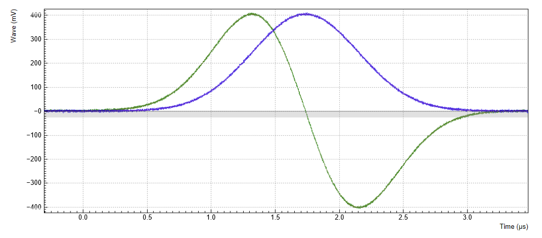
While the AWG is running, you can enable modulation by setting the AWG channel 1 Modulation to Sine 11, and AWG channel 2 Modulation to Sine 22. The notation Sine NM with N, M = 1, 2,... signifies the following: the given AWG channel is multiplied with the signal of Sine Generator N when routed to the first Wave output of the given AWG core, and with the signal of Sine Generator M when routed to the second Wave output of the given AWG core. Here, we route the AWG signals only along the diagonal path (AWG channel 1 to Wave 1, and AWG channel 2 to Wave 2), so we make use of only 2 of the 4 signal multipliers of core 1. The resulting signal on Wave 1 is AWG1×Sine1, and the resulting signal on Wave 2 is AWG2×Sine2. Here, AWG1 denotes the signal of AWG channel 1 (the Gaussian pulse) AWG2 the signal of AWG channel 2 (the DRAG pulse), and Sine1 (Sine2) the signal of Sine Generator 1 (2).
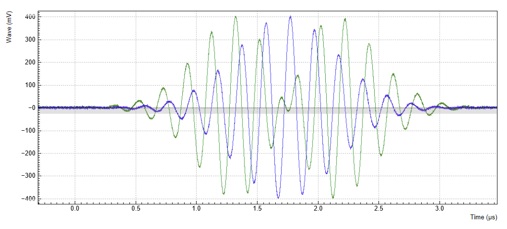
The lower plot in Figure 2 shows the resulting signals, which are the Gaussian and DRAG pulses multiplied by a 5 MHz carrier with phase shift 0° and 90°, respectively.
| Tab | Sub-tab | Section | # | Label | Setting / Value / State |
|---|---|---|---|---|---|
| Output | Waveform Generators | 1 | Modulation | Sine 11 | |
| Output | Waveform Generators | 2 | Modulation | Sine 22 |
In this practical case of I/Q modulation, the two Wave outputs typically require further adjustments of the pulse amplitude, DC offset, and inter-channel phase offset in order to compensate for analog mixer imperfections. All these adjustments can now be done on the fly using the AWG Amplitude, the Wave Output Offset, and the Sine Generator Phase settings without having to make any changes to the programmed AWG waveforms.
For certain cases of I/Q modulation, it’s required to generate linear
combinations of 2 modulated signal on each Wave output. To realize this,
we can make use of all 4 signal multipliers of the AWG core. We can
modify the sequence program such that each AWG channel is routed to both
Wave outputs by passing additional arguments to the playWave
instruction (see
Multi-Channel Playback):
wave w_gauss = gauss(8000, 4000, 1000);
wave w_drag = drag(8000, 4000, 1000);
while (true) {
    setTrigger(1);
    playWave(1, 2, w_gauss, 1, 2, w_drag);
    waitWave();
    setTrigger(0);
    wait(100);
}
In a typical case, we want to use crossed assignments between AWG channels and Sine generators by selecting the settings in the following table. In order to prevent an overflow condition of the summed-up signals, we set the gain parameters at each signal multiplier to 0.5.
| Tab | Sub-tab | Section | # | Label | Setting / Value / State |
|---|---|---|---|---|---|
| Output | Waveform Generators | 1 | Modulation | Sine 12 | |
| Output | Waveform Generators | 2 | Modulation | Sine 21 | |
| Output | Waveform Generators | 1 | Output Amplitude Wave 1 | 0.5 | |
| Output | Waveform Generators | 1 | Output Amplitude Wave 2 | 0.5 | |
| Output | Waveform Generators | 2 | Output Amplitude Wave 1 | 0.5 | |
| Output | Waveform Generators | 2 | Output Amplitude Wave 2 | 0.5 |
With these settings and the above sequence program, the resulting signal on Wave 1 is equal to AWG1×Sine1 + AWG2×Sine2, and the resulting signal on Wave 2 is equal to AWG1×Sine2 + AWG2×Sine1.
Rapid Phase Changes
The HDAWG supports rapid, real-time changes of the carrier phase in
modulation mode through the sequencer instructions setSinePhase and
incrementSinePhase. This capability is particularly valuable when
generating long patterns of pulses with varying phases, e.g. to account
for AC Stark shift in qubit control sequences, or to realize phase
cycling protocols.
In addition, there is the possibility to reset the starting phase of one
or multiple oscillator at the beginning of a pulse sequence using the
resetOscPhase instruction. Thus it can be ensured that the
carrier-envelope offset, and thus the final output signal, is identical
from one repetition to the next.
Due to the architecture of the HDAWG, both the Sine Generators and the
Oscillators are physically located in the front-end FPGAs of the
instrument (see
AWG Architecture and Execution Timing).
For instruments with the HDAWG-MF option, each of the 8 or 16 oscillator
exists as a copy on each front-end FPGA. When changing an oscillator
frequency from the graphical user interface, all copies get
synchronously updated to the new configuration with the help of the
back-end FPGA. This synchronization mechanism is however relatively slow
and not a real-time operation. When making use of the fast oscillator
control in the form of the resetOscPhase instruction, the
synchronization mechanism needs to be turned off by enabling the AWG
Oscillator Control mode. Each AWG core is then allowed to control and
use only a subset of oscillators: Oscillators 1 through 4 on core 1,
oscillators 5 through 8 on core 2, and so forth. In the following
example, we will use the oscillator 1 for both Sine Generators on AWG
core 1. On instruments without the HDAWG-MF option, this is the default
configuration and not modifiable. Apply the settings in the following
table.
| Tab | Sub-tab | Section | # | Label | Setting / Value / State |
|---|---|---|---|---|---|
| Output | Waveform Generators | 1 | Modulation | Sine 11 | |
| Output | Waveform Generators | 2 | Modulation | Sine 22 | |
| Output | Sine Generators | 1 | Osc | 1 | |
| Output | Sine Generators | 2 | Osc | 1 | |
| Output | Oscillators | AWG Oscillator Control | ON |
In the following AWG sequencer program, we generate a series of 4
dual-channel square pulses that are played back-to-back. We initialize
the oscillator phase by a resetOscPhase instruction. In this form
without an argument, the instruction will reset the phases of all
oscillators accessible by this core (here oscillators 1 through 4).
Alternatively, an argument in binary representation, e.g. 0b0101,
allows us to reset only a subset of these oscillators. We then set the
phases of sine generators 1 and 2 to zero using the setSinePhase
instruction. Subsequently, we play back the dual-channel waveform 4
times, and after each playback instruction, we increase the phase of
sine generator 2 by 60 degrees. The corresponding instruction
incrementSinePhase takes effect at the end of the previous waveform
playback, which allows us to change the phase precisely in between
waveforms. Upload the following sequence program to the AWG and run the
sequence.
wave w_pulse = ones(800);

while (true) {
  // generate trigger for scope
  setTrigger(1);
  setTrigger(0);
  // initialize oscillator frequency, reset phase
  wait(100);
  resetOscPhase();
  setSinePhase(0, 0);
  setSinePhase(1, 0);
  wait(100);

  // play waveform and change sine generator phase
  playWave(w_pulse, w_pulse);

  incrementSinePhase(1, 60); // phase increment takes effect at the end
                             // of the previous waveform
  playWave(w_pulse, w_pulse);
  incrementSinePhase(1, 60); // phase increment takes effect at the end
                             // of the previous waveform
  playWave(w_pulse, w_pulse);
  incrementSinePhase(1, 60); // phase increment takes effect at the end
                             // of the previous waveform
  playWave(w_pulse, w_pulse);
  wait(10000);
}
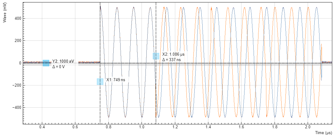
The resulting signal shown in Figure 3 nicely shows how the relative phase of the two signal, starting out at 0, incrementally changes in steps of 60 degrees. The end of the first waveform is marked by a cursor. In the 4th waveform, the two carrier signals are offset by exactly 180 degrees.
Note
The phase increment due to the incrementSinePhase instruction takes
effect at the end of the previous waveform playback. In case the
instruction is placed in the sequencer code before the first playWave
instruction, the phase increment will only happen after the playWave
instruction.
Multi-frequency Modulation
When the HDAWG-MF Multi-frequency option is installed, the HDAWG supports modulation of multiple carriers with individual envelope signals. This technique allows us to generate signals which, using conventional sample-by-sample waveform programming, would require to store thousands of waveforms instead of just one envelope waveform. Typical use cases are phase cycling protocols in NMR spectroscopy, or frequency-multiplexing techniques. The latter requires the HDAWG-MF option, whereas the former requires only the base instrument. Multi-carrier modulation is realized by four-fold interleaving of one AWG channel and individual multiplication of the four channels with one of the oscillator signals. The envelope sampling rate is therefore reduced by a factor of 4, whereas the carrier signal is still generated at the full sampling rate, therefore giving access to the full bandwidth.
With the following sequence program, we generate a series of pulses with
changing carrier. The first four pulses each have a single carrier
coming from one of the first four oscillators. In the fifth pulse, all
carrier signals are superimposed. The interleave instruction, which we
use several times, allows us to combine four waveforms into one.
const n_samples = 512;
wave w_gauss = 0.25*gauss(n_samples, n_samples/2, n_samples/10);
wave w_zeros = zeros(n_samples);

wave w_channel_1 = interleave(w_gauss, w_zeros, w_zeros, w_zeros);
wave w_channel_2 = interleave(w_zeros, w_gauss, w_zeros, w_zeros);
wave w_channel_3 = interleave(w_zeros, w_zeros, w_gauss, w_zeros);
wave w_channel_4 = interleave(w_zeros, w_zeros, w_zeros, w_gauss);
wave w_all_channels = interleave(w_gauss, w_gauss, w_gauss, w_gauss);

while (true) {
  playWave(w_channel_1);
  playWave(w_channel_2);
  playWave(w_channel_3);
  playWave(w_channel_4);
  setTrigger(1);
  setTrigger(0);
  playWave(w_all_channels);
  playZero(n_samples); //spacing between pulses
}
In the Multi-frequency modulation tab, we route the oscillator signals 1 to 4 to the AWG Output 1 Modulation sine generators 1 to 4 by changing the selectors in the Osc column. We set the frequencies of oscillators 1 to 4 in the Output tab to mutually different values. Deliberately, we offset oscillator 4 frequency by 1 Hz from a round value to 40.000001 MHz. This helps us demonstrate that the phase coherence is maintained independently by all oscillators. Finally, in the Output tab we set Modulation to Advanced.
| Tab | Sub-tab | Section | # | Label | Setting / Value / State |
|---|---|---|---|---|---|
| Output | Oscillators | 1 | Frequency | 10 MHz | |
| Output | Oscillators | 2 | Frequency | 20 MHz | |
| Output | Oscillators | 3 | Frequency | 30 MHz | |
| Output | Oscillators | 4 | Frequency | 40.000001 MHz | |
| MF Mod | AWG Output 1 Modulation | 1 | Osc | 1 | |
| MF Mod | AWG Output 1 Modulation | 2 | Osc | 2 | |
| MF Mod | AWG Output 1 Modulation | 3 | Osc | 3 | |
| MF Mod | AWG Output 1 Modulation | 4 | Osc | 4 | |
| Output | Waveform Generators | 1 | Modulation | Advanced |
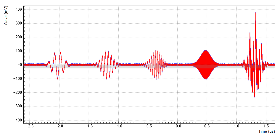
Figure 4 shows the signal captured by the scope after having made all the settings and uploaded and played the sequence program above. In the first three pulses (10, 20, and 30 MHz) the phase is stable because the repetition rate is commensurate with the carrier frequencies. The fourth pulse (40.000001 MHz) and the fifth pulse (sum of all carriers) vary their shape over time, which is made visible by enabling scope persistence. As mentioned in the beginning, generating such a signal conventionally would consume a much larger amount of waveform memory.