Pulse-level sequencing with the Command Table
Goals and Requirements
The goal of this tutorial is to demonstrate pulse-level sequencing using the command table feature of the HDAWG.
Preparation
Connect the cables as illustrated below. Make sure that the instrument is powered on and connected by Ethernet to your local area network (LAN) in which the control computer resides. After starting LabOne, the default web browser opens with the LabOne graphical user interface. The tutorial can be started with the default instrument configuration (e.g. after a power cycle) and the default user interface settings (e.g. as is after pressing F5 in the browser). Additionally, this tutorial requires the use of one of our APIs, in order to be able to define and upload the command table itself. The examples shown here use the Python API, similar functionality is available also for C++, Matlab and .Net.

Introduction to the Command table
The command table allows the sequencer to group waveform playback
instructions with other timing-critical phase and amplitude setting
commands in a single instruction within one clock cycle of 3.33 ns. The
command table is a unit separate from the sequencer and waveform memory.
Both the phase and the amplitude can be set in absolute and in
incremental mode. Even when not using digital modulation or amplitude
settings, working with the command table has the advantage of being more
efficient in sequencer instruction memory compared to standard
sequencing. Starting a waveform playback with the command table always
requires just a single clock cycle, as opposed to 2 or 3 when using a
playWave instruction.
When using the command table, three components play together during
runtime to generate the waveform output and apply the phase and
amplitude setting instructions:
- Sequencer: the unit executing the runtime instructions, namely in this
context the executeTableEntry instruction. This instruction executes
one entry of the command table, and its input argument is a command
table index. In its compiled form which can be seen in the AWG
Sequencer Advanced sub-tab, the sequence program can contain up to
16384 instructions.
- Wave table: a list of up to 16000 indexed waveforms. This list is
defined by the sequence program using the index assignment instruction
assignWaveIndex combined with a waveform or waveform placeholder.
The wave table index referring to a waveform can be used in two ways:
it is referred to from the command table, and it is used to directly
write waveform data to the instrument memory using the node
/<dev>/AWGS/<n>/WAVEFORM/WAVES/<index>
- Command table: a list of up to 1024 indexed entries (command table
index), each containing the index of a waveform to be played (wave
table index), a sine generator phase setting instruction, and an AWG
amplitude setting instruction. The command table is specified by a
JSON formatted string written to the node
/<dev>/AWGS/<n>/COMMANDTABLE/DATA
Basic command table use
We start in Python by defining a sequencer program that uses the command table.
seqc_program = """\
  // Define two waveforms
  wave w_a = gauss(2048, 1, 1024, 256);
  wave w_b = gauss(2048, 1, 1024, 192);

  // Assign a dual channel waveform to wave table entry 0
  assignWaveIndex(w_a, w_b, 0);

  // execute the first command table entry
  executeTableEntry(0);
  // execute the second command table entry
  executeTableEntry(1);
"""
It defines two Gaussian waveforms of equal amplitude and total length, but different width. These waveforms are then assigned as to two channels of the wave table entry with index 0, and the final lines executes the two first command table entries. This program cannot be run yet, as the command table is not yet defined, this is done in the next step. The command table must be uploaded after the sequence and never before.
Note
If a sequence program contains a reference to a command table entry that has not been defined, or if a command table entry refers to a waveform that has not been defined, the sequence program can’t be run.
In general the command table is defined as a JSON formatted string.
Below we show an example of how to define a command table with two
entries using Python. For ease of programming, here we define the
command table as a CommandTable object, which is converted into a JSON
string automatically at upload. Such object also validate the fields of
the command table.
In this example, we generate a first command table entry with index "TABLE_INDEX", which plays the dual-channel waveform referenced in the wave table at index "WAVE_INDEX", with amplitude and phase settings specified for both channels individually. The second command table entry plays the same waveform again, but only sets the amplitude for the first output channel.
Here the Python code that uploads both the previously defined sequence and the command table.
## Imports
## Load the LabOne API and other necessary packages
from zhinst.toolkit import Session, CommandTable

device_id='dev8000'
server_host = 'localhost'
### connect to data server
session = Session(server_host)
### connect to device
device = session.connect_device(device_id)

AWG_INDEX = 0 # which AWG core to be used, here: first two channels
awg = device.awgs[AWG_INDEX]

## Load the sequence
awg.load_sequencer_program(seqc_program)

## Initialize command table
ct_schema = awg.commandtable.load_validation_schema()
ct = CommandTable(ct_schema)

## Index of wave table and command table entries
TABLE_INDEX = 0
WAVE_INDEX = 0

## Waveform with amplitude and phase settings
ct.table[TABLE_INDEX].waveform.index = WAVE_INDEX
ct.table[TABLE_INDEX].amplitude0.value = 1.0
ct.table[TABLE_INDEX].amplitude1.value = -0.5
ct.table[TABLE_INDEX].phase0.value = 0
ct.table[TABLE_INDEX].phase0.increment = False
ct.table[TABLE_INDEX].phase1.value = 90
ct.table[TABLE_INDEX].phase1.increment = False

ct.table[TABLE_INDEX+1].waveform.index = WAVE_INDEX
ct.table[TABLE_INDEX+1].amplitude0.value = 0.5

## Upload command table
awg.commandtable.upload_to_device(ct)
Note
During compilation of a sequencer program, any previously uploaded command table is reset, and will need to be uploaded again before it can be used.
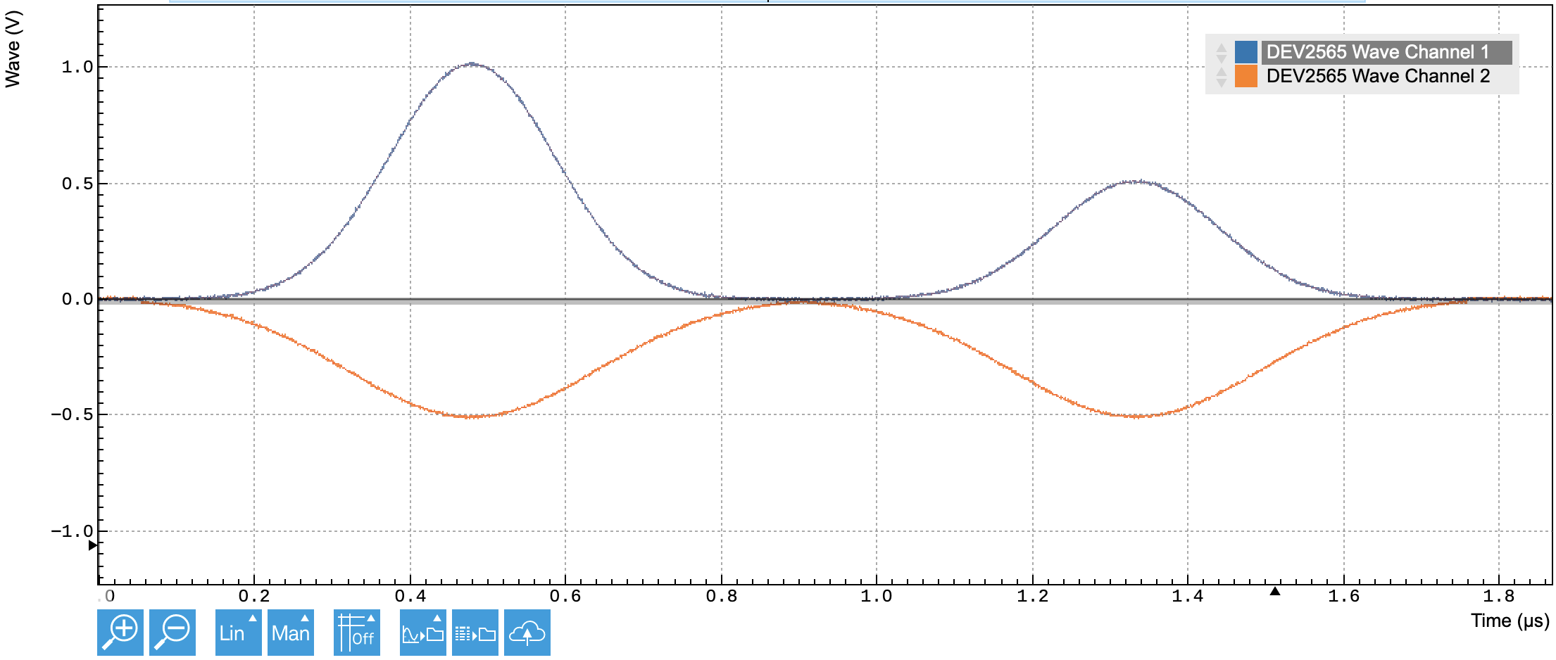
Now the sequencer program can be run on the HDAWG. The expected output is shown in Figure 2. Note how the amplitude of the Gaussian waveform played on the second channel is negative and half the magnitude of the waveform on the first channel, even though they are both defined with the same amplitude in the sequencer program. This is due to the amplitude settings in the command table. Also note that these amplitude settings are persistent, as in the second command table entry, the amplitude of the first output channel is set to 0.5, while the second channel remains as in the previous playback.
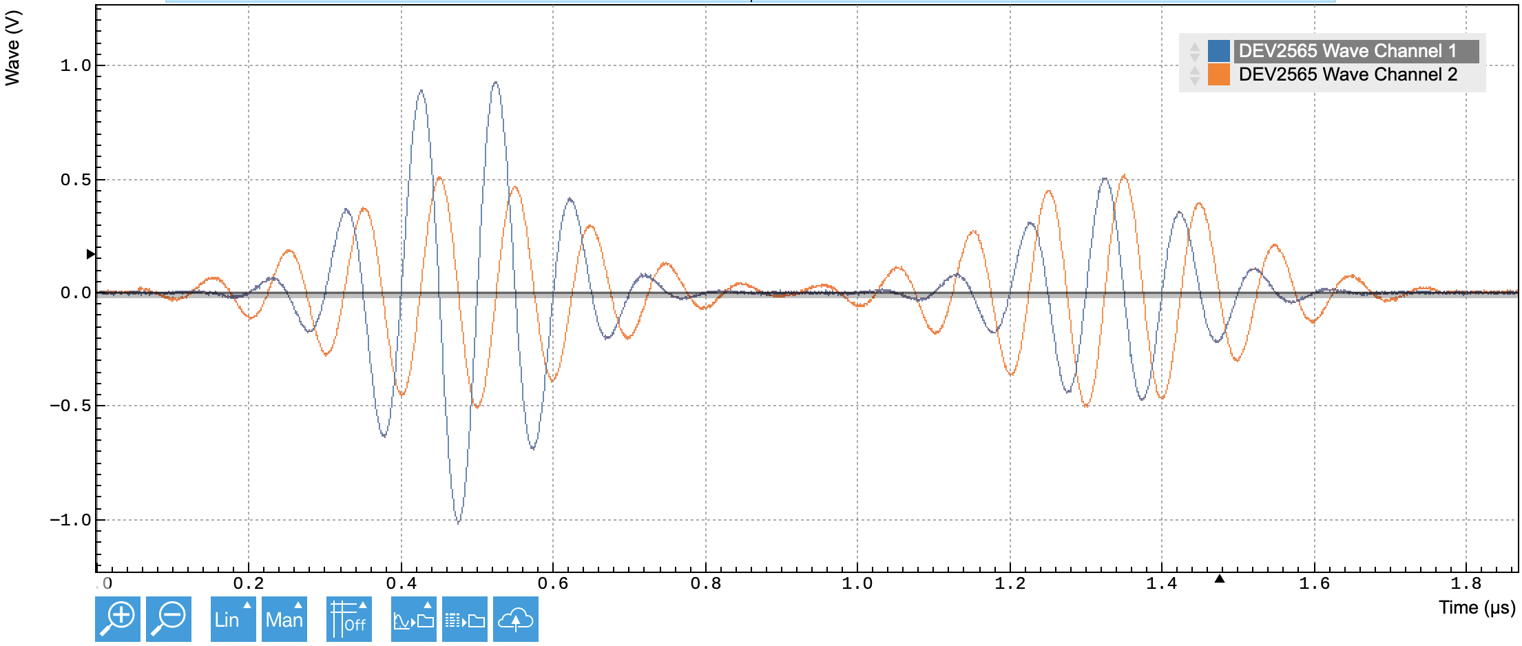
The phase settings we specified in the definition of the command table have no immediate impact on the output waveforms we show here, since we have not yet added digital modulation. Enabling digital modulation for the two output channels used here, with the same frequency and sine generator phase for both channels, the expected output is now shown in Figure 3. Note the phase offset between the two channels, due to the phase increment of 90 degrees for the second channel in the command table.
Note
When a command table entry is called, the amplitude and phase are set persistently. Subsequent waveforms on the same channel will be played with the same amplitude and phase. To play a waveform with a different amplitude or phase, the new values must be set with another command table entry.
Phase entries in the command table supersede any settings in the GUI. In the presence of a command table, the phase of sine generators is reset to zero when enabling the sequencer. To apply a non-zero phase to the sine generators in the presence of a command table, the phase must either be set within the command table itself or with the setSinePhase sequencer command.
Efficient pulse incrementation
One illustrative use case of the command table feature is the efficient incrementation of amplitude or phase of waveforms.
We again start by writing a sequencer program that plays two entries of the command table.
seqc_program = """\
  // Define a single waveform
  wave w_a = ones(1024);

  // Assign a dual channel waveform to wave table entry
  assignWaveIndex(w_a, w_a, 0);

  // execute the first command table entry
  executeTableEntry(0);
  repeat(10) {
    executeTableEntry(1);
  }
"""
Here we have defined a single wave table entry, where both channels contain the same constant waveform.
In Python we then define and upload a command table with just two entries, in this case both referencing the same wave table entry.
## Load the sequence
awg.load_sequencer_program(seqc_program)

## Initialize command table
ct_schema = awg.commandtable.load_validation_schema()
ct = CommandTable(ct_schema)

## Waveform with amplitude and phase settings
ct.table[0].waveform.index = 0
ct.table[0].amplitude0.value = 1.0
ct.table[0].amplitude1.value = 0.0

ct.table[1].waveform.index = 0
ct.table[1].amplitude0.value = -0.1
ct.table[1].amplitude0.increment = True
ct.table[1].amplitude1.value = 0.1
ct.table[1].amplitude1.increment = True

## Upload command table
awg.commandtable.upload_to_device(ct)
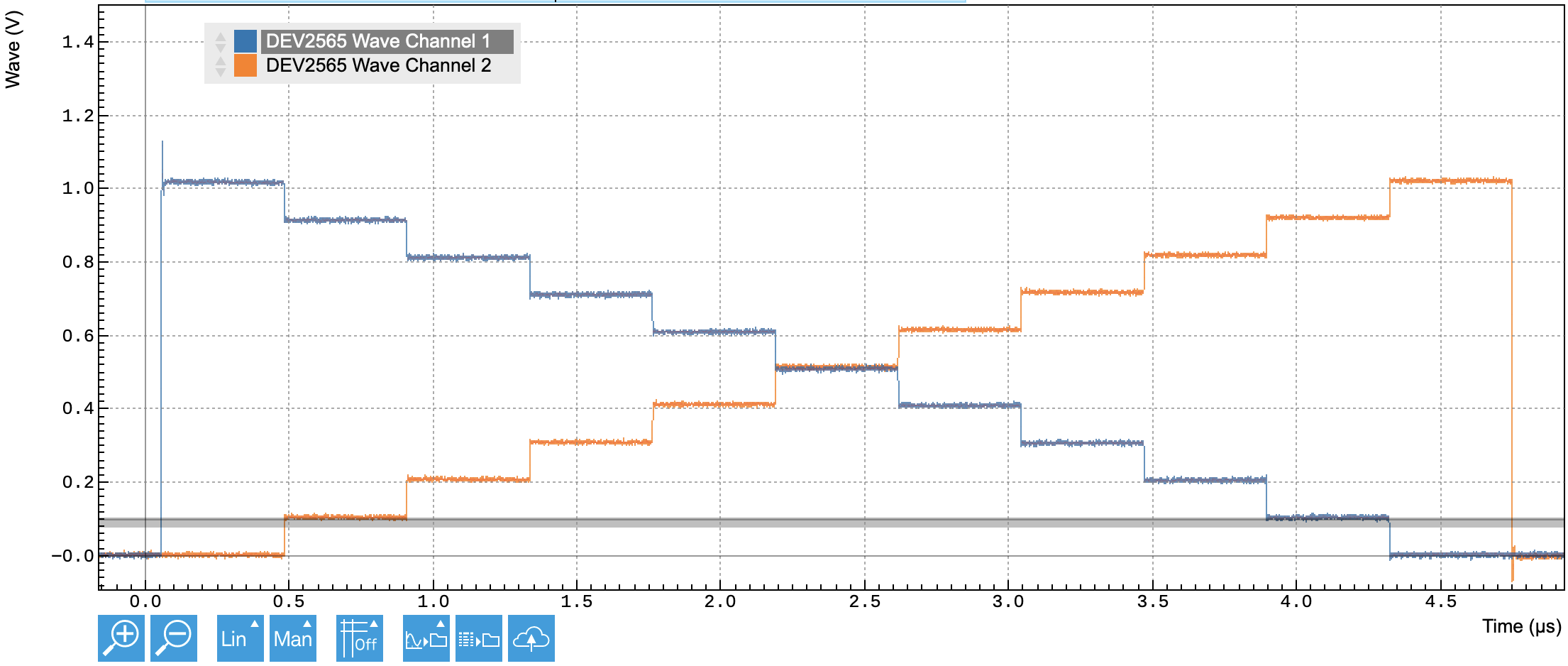
Executing the sequencer program then produces the two-channel output shown in Figure 4. Here, the first call to the first command table entry plays the two-channel waveform with the amplitude of the first output channel set to one and for the second channel set to zero. The subsequent calls to the second command table entry increment these amplitudes every time by 0.1, with a negative increment on channel 1, and an positive increment on channel 2.
Note
The amplitude of waveform playback can be influenced in multiple different ways, through the amplitude of the waveform itself, through the amplitude setting in the command table, and finally through the Range setting of the AWG output channel.
It is possible to perform multi-dimensional amplitude sweeps by making use of the amplitude registers of the command table. Each channel has four independent amplitude registers, with each register storing the amplitude last played on that register. By default, amplitude register zero is used. It is therefore possible to keep the amplitude of one register constant while sweeping the amplitude of another register. This can be useful for probing dynamics in a multi-level system, or for certain steps in the calibration of spin qubits.
As an example, we will use the following sequence:
seqc_program = """\
    assignWaveIndex(ones(128), 0);
    assignWaveIndex(rect(64,0.2), 1);

    var i = 10;
    executeTableEntry(0);
    do {
        executeTableEntry(2);
        executeTableEntry(1);
        i-=1;
    } while(i);
"""

## Upload the sequence
awg.load_sequencer_program(seqc_program)
The first executeTableEntry command initializes the amplitude that
will be swept without playing a pulse. The second executeTableEntry
plays a constant rectangular pulse (64 samples long, amplitude 0.2). The
third executeTableEntry plays a rectangular pulse (128 samples long)
whose amplitude will be swept. The loop will play 10 different
amplitudes. We also need to define and upload a command table to go with
the sequence:
## Initialize command table
ct_schema = awg.commandtable.load_validation_schema()
ct = CommandTable(ct_schema)
## Initialize amplitude register 1
ct.table[0].amplitude0.value = -0.8
ct.table[0].amplitude0.increment = False
ct.table[0].amplitude0.register = 1
## Swept rectangular pulse
ct.table[1].waveform.index = 0
ct.table[1].amplitude0.value = 0.15
ct.table[1].amplitude0.increment = True
ct.table[1].amplitude0.register = 1
## Constant rectangular pulse
ct.table[2].waveform.index = 1
ct.table[2].amplitude0.value = 1.0
ct.table[2].amplitude0.register = 0

## Upload command table
awg.commandtable.upload_to_device(ct)
The first command table entry (index 0) sets the initial amplitude (in this case, -0.8) of amplitude register 1. The second table entry (index 1) increments the amplitude of amplitude register 1 and plays the rectangular pulse with waveform index 0. The third table entry (index 2) plays the constant rectangular pulse (waveform index 1) using amplitude register 0.
We now run the sequence:
awg.enable(True)
We observe the signal shown in Figure 5, which shows a constant pulse of 100 mV interleaved with a pulse whose amplitude is swept in steps of 75 mV. In total, there are 10 different amplitudes of the swept pulse.

Pulse-level sequencing with the command table
All previous examples have used the pulse library in the AWG sequencer to define waveforms. In more advanced scenarios, waveforms are uploaded through the API, as we will demonstrate next. We start with the following sequence program, where we assign wave table entries using the placeholder command with a waveform length as argument.
seqc_program = """\
  // Define two wave table entries through placeholders
  assignWaveIndex(placeholder(1024), placeholder(1024), 0);
  assignWaveIndex(placeholder(1024), placeholder(1024), 1);

  // execute command table
  executeTableEntry(0);
  executeTableEntry(1);
  executeTableEntry(2);
"""

## Upload the sequence
awg.load_sequencer_program(seqc_program)
In this form, the sequence program cannot be run, first because the command table is not yet uploaded, and second because the waveform memory in the wave table has not been defined. We can use the numpy package to define two-channel Gaussian waveforms directly in Python, and upload them to the instrument using the appropriate node.
from zhinst.toolkit import Waveforms
import numpy as np

## parameters for waveform generation
length = 1024
width = 1/4
x = np.linspace(-1, 1, length)

## define waveforms as list of real-values arrays - here: Gaussian functions
waves = [
    [np.exp(-x**2/width**2), np.zeros(length)],
    [np.zeros(length), np.exp(-x**2/width**2)]]

## Upload waveforms to instrument
waveforms = Waveforms()
for i, wave in enumerate(waves):
  waveforms[i] = (wave[0],wave[1])
awg.write_to_waveform_memory(waveforms)
Finally, we also generate and upload a command table to the instrument.
## Initialize command table
ct_schema = awg.commandtable.load_validation_schema()
ct = CommandTable(ct_schema)

## Waveform with amplitude and phase settings
ct.table[0].waveform.index = 0
ct.table[0].waveform.awgChannel0 = ["sigout0"]
ct.table[0].waveform.awgChannel1 = ["sigout1"]
ct.table[0].amplitude0.value = 1.0
ct.table[0].amplitude1.value = -1.0

ct.table[1].waveform.index = 1
ct.table[1].waveform.awgChannel0 = ["sigout1"]
ct.table[1].waveform.awgChannel1 = ["sigout0"]

ct.table[2].waveform.index = 1
ct.table[2].waveform.awgChannel0 = ["sigout0","sigout1"]
ct.table[2].waveform.awgChannel1 = ["sigout0","sigout1"]

## Upload command table
awg.commandtable.upload_to_device(ct)
The sequencer program can now be run, and will produce output as shown in Figure 6.
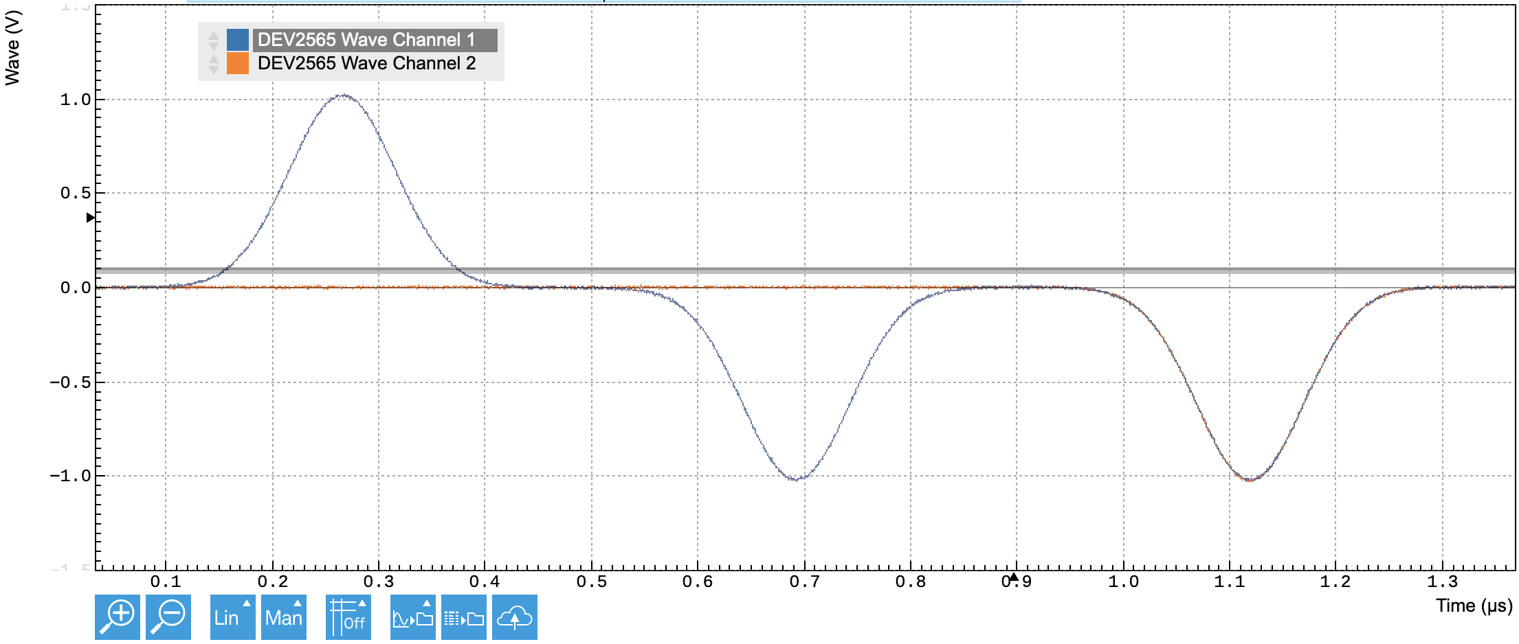
Here, the playback of the first command table entry plays the first waveform with the standard output channel assignment. It also sets the amplitude of the second output channel to -1.0, even though no signal is played on this channel. The second command table playback plays the second wave table entry, but with the output assignment switched, meaning channel 1 is played on output 2 and vice versa. Due to the amplitude settings in the first command table entry, the waveform defined for channel 2 is played with a negative amplitude. The final command table entry again plays the second entry of the wave table, now with both channels assigned to both outputs, and therefore results in the same waveform played on both outputs. This last setting would typically be used when using IQ upconversion to convert the HDAWG signal to RF frequencies, as demonstrated in the previous tutorial chapter.
Command table entries fields
The documentation of all possible parameters in the command table JSON
file can be found by pulling the schema from the device itself using the
node /<dev>/AWGS/<n>/COMMANDTABLE/SCHEMA. The Python CommandTable
object automatically uses the schema from the device when initialized
like this:
## Initialize command table
ct_schema = awg.commandtable.load_validation_schema()
ct = CommandTable(ct_schema)
Table 1 contains all
elements that can be programmed as part of a command table entry as well
as the default value which is applied if this element is not specified
by the user. Table 2 contains
all parameters of a waveform element, as well as each parameter’s
default value. Analogously,
Table 3 contains the
parameters of a phase type element (phase0, phase1), and
Table 4 those of an amplitude
type entry (amplitude0 or amplitude1).
If a phase element is specified in any entry of the command table, the absolute phase will be set to zero at the start of the execution, while the amplitudes are set to one.
| Field | Description | Type | Range/Value | Mandatory | Default |
|---|---|---|---|---|---|
| index | Index of the entry | Integer | [0—1023] | yes | mandatory |
| waveform | Waveform command and its properties | Waveform | no | No waveform played | |
| phase0 | Phase command for the first AWG channel | Phase | no | No change to phase setting | |
| phase1 | Phase command for the second AWG channel | Phase | no | No change to phase setting | |
| amplitude0 | Amplitude command for the first AWG channel | Amplitude | no | No change to amplitude setting and amplitude register set to 0 | |
| amplitude1 | Amplitude command for the second AWG channel | Amplitude | no | No change to amplitude setting and amplitude register set to 0 |
| Field | Description | Type | Range/Value | Mandatory | Default |
|---|---|---|---|---|---|
| index | Index of the waveform to play as defined with the assignWaveIndex sequencer instruction |
integer | [0—15999] | if playZero or playHold is False | No waveform played |
| length | The length of the waveform in samples | integer | [32—WFM_LEN] | if playZero or playHold is True | the waveform length as declared in the sequence |
| samplingRate Divider |
Integer exponent n of the sampling rate divider: SampleRate / 2n | integer | [0—13] | no | 0 |
| awgChannel0 | Assign the first AWG channel to signal outputs | list | {"sigout0","sigout1"} | no | The channel assignment declared in assignWaveIndex |
| awgChannel1 | Assign the second AWG channel to signal outputs | list | {"sigout0","sigout1"} | no | The channel assignment declared in assignWaveIndex |
| precompClear | Set to true to clear the precompensation filters | bool | [True,False] | no | False |
| playZero | Play a zero-valued waveform for specified length of waveform | bool | [True,False] | no | False |
| playHold | Hold the value of the last waveform and marker sample played for specified length | bool | [True,False] | no | False |
| Field | Description | Type | Range/Value | Mandatory | Default |
|---|---|---|---|---|---|
| value | Phase value of the given sine generator in degree | float | [-180.0—180.0) values outside of this range will be clamped | Yes | mandatory |
| increment | Set to true for incremental phase value, or to false for absolute | bool | [True,False] | No | False |
| Field | Description | Type | Range/Value | Mandatory | Default |
|---|---|---|---|---|---|
| value | Amplitude scaling factor of the given AWG channel | float | [-1.0—1.0] | If register is absent | 1.0 or previous value in the register |
| increment | Set to true for incremental amplitude value, or to false for absolute | bool | [True,False] | No | False |
| register | Index of amplitude register that is selected for scaling the pulse amplitude. | integer | [0—3] | If value is absent | 0 |