Precompensation Tab
The Precompensation tab relates to the HDAWG-PC Real-time Precompensation option and is only available if this option is installed on the instrument (see Information section in the Device tab).
Features
- Real-time waveform processing for in-situ tunability
- High-pass compensation
- Overshoot/undershoot compensation with 8 exponential filters
- Bounce compensation for reflections and standing waves
- Programmable FIR filter with convolution length 30 ns
- Precompensation Simulator
- Latency calculation
- Filter reset by AWG sequence instruction
Description
The Precompensation tab provides access to the real-time precompensation filter configuration and the Precompensation Simulator. Whenever the tab is closed, clicking the following icon will open a new instance of the tab.
| Control/Tool | Option/Range | Description |
|---|---|---|
| Precompensation | Configure the Real-time Precompensation filters. |
The Precompensation tab shown in Figure 1 consists of a configuration section on the left and a display section on the right. The configuration section is further divided into a subsection for device parameters on the left, and for simulation parameters on the right.
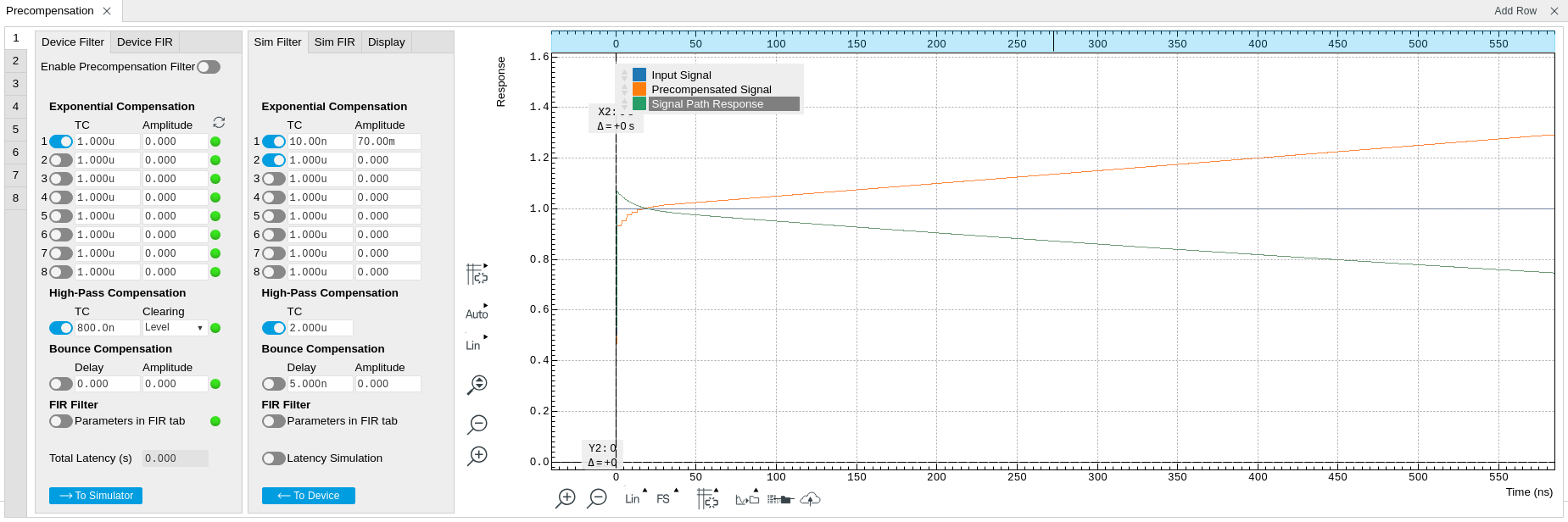
There is one precompensation unit for each Wave output of the HDAWG. The individual units are represented as numbered side-tabs. Each unit consists of a chain of filters represented in the Device Filter tab. The filter chain is shown as a flow diagram in Figure 2 and consists of 8 exponential compensation filters, 1 high-pass compensation filter, 1 bounce compensation filter, and 1 FIR filter. All configurable filter parameters are represented as rows in the Device Filter tab, with the exception of the FIR filter parameters which are located in the separate Device FIR sub-tab. The entire filter chain can be bypassed or enabled with the Enable Precompensation Filter button, and each filter can be enabled using a button on the left side of the corresponding filter settings. The filter parameters are explained in the following section.
The right side of the configuration section as well as the display section represent the Precompensation Simulator. The Precompensation Simulator is a software-based tool to accurately model the hardware filter and thus allows one to find suitable filter parameters based on a step response measurement of the external circuit. The display section shows three simulated step response curves based on the currently s parameters in the Sim Filter sub-tab:
- Input signal : this curve represents an ideal step signal for reference
- Precompensated signal : this curve represents the simulated output
of the precompensation unit, when the AWG generates a step signal as
an input to the precompensation unit, e.g. using a sequencer
instruction
playWave(ones(10000)). The precompensated signal approximately equals the signal expected at the Wave output of the HDAWG with enabled precompensation filter, apart from distortions introduced by the analog output stage of the HDAWG. - Signal path response: this curve represents the step response of the inverse of the precompensation filter. This is the step response of a hypothetical signal path that the currently simulated filter would ideally compensate.
Note
The precompensated signal generated by the hardware is limited by the DAC full scale. If the Simulator Input Signal is chosen to be equal to the AWG output (including digital AWG gain factors) and the Simulator Precompensated Signal absolute value exceeds 1, an overflow condition is to be expected at the DAC. The overflow condition is then indicated by a red filter status LEDs when enabling the precompensation filter. This condition is to be avoided by either adjusting the filter parameters, or rescaling the AWG output signal.
In a typical workflow, the user would start by a measurement of the step response of the full signal path from the AWG to the reference point at the device under test. Often this can be achieved by an averaged oscilloscope measurement at the reference point while generating a step signal with the AWG with disabled precompensation filter, e.g. using the following sequence program:
const plateau_width = 10e-6;
const wait_time = 10e-3;
const amplitude = 0.5;

while (true) {
  // Plays a square pulse with high-pass precompensation filter active
  setPrecompClear(0);
  playWave(amplitude*ones(plateau_width*DEVICE_SAMPLE_RATE));

  // Plays a short zero-waveform and reset the high-pass precompensation filter
  setPrecompClear(1);
  playWave(zeros(32));

  // Wait time
  playZero(wait_time*DEVICE_SAMPLE_RATE);
}
Consider the following points when using this sequence program:
- The step signal amplitude (here 0.5) should be less than 1.0 in order to provides the digital-to-analog converter with a certain headroom to avoid overflow in case the filter generates positive corrections. This is always the case for the high-pass compensation filter.
- The timescale of the plateau width (here 10 µs) should correspond the timescale of the final signals, and should notably be shorter than a possible high-pass filter time constant in the signal path.
- The waiting time between pulses (here 10 ms) should be much larger than a possible high-pass filter time constant in the signal path, such that there are no history effects.
- The
setPrecompClear(1)instruction together with the subsequent playback of a zero-valued waveformplayWave(zeros(32))ensures that the precompensation filters are reset after the measurement, to prevent history effects.
In the next step, the user would adjust the simulator filter parameters such that the displayed signal path response curve matches the measured step response as closely as possible. The measurement graphs shown in the following section may help to visually identify which type of filter applies to a given signal characteristic observed in the step response measurement.
Once satisfied with the result, the simulation parameters can be
transferred to the hardware filters by clicking on  .
The step response measurement described above can then be repeated, this
time with enabled precompensation filter. At this stage, fine
adjustments of the enabled filters can be done while observing their
effect on the signal.
.
The step response measurement described above can then be repeated, this
time with enabled precompensation filter. At this stage, fine
adjustments of the enabled filters can be done while observing their
effect on the signal.
After having eliminated the largest signal distortions, smaller exponential overshoots or undershoots may now become measurable. Iteratively, one can now enable additional exponential filters in order to suppress these.
In case that the GUI-based procedure described here does not yield sufficiently accurate results, consider using a systematic numeric optimization using the one of LabOne APIs in order to exploit the full potential of the HDAWG-PC Real-time Precompensation. Please refer to the documentation of the Precompensation Module in the LabOne Programming Manual. The LabOne Python API comes with an example implementation of a numeric filter optimization.

Latency and Status
Enabling the full filter chain leads to a signal processing latency of 9
filter clock cycles, where the filter clock runs at 1/8 of the sampling
clock. With a sampling clock rate of 2.4 GSa/s, the filter clock
frequency is 2400/8 MHz = 300 MHz and the minimum latency is 9/(300 MHz)
= 30 ns. Each filter of the chain adds an additional latency when it is
enabled, as specified by the red numbers in Figure 2. The total
latency caused by the current filter configuration is displayed at the
bottom of the Device Filter sub-tab. Each filter has a Status LED on the
right side of the settings. A red LED indicates that an arithmetic
overflow currently occurs, while a yellow LED indicates that an overflow
occurred in the past. The status of all filters can be cleared with the
 button. An overflow occurs if the output of the precompensation filter
reaches the maximum or minimum of the digital-to-analog converter range.
The reason for an overflow can often be diagnosed by inspecting the
precompensated signal in the simulator, and can often be eliminated by
adjusting the AWG signal. Be aware that an overflow may also hint at the
fact that a desired precompensation is not physically realizable. For
example, it is not possible to apply a high-pass compensation to a
square signal which is already at the maximum output voltage of the
instrument, as this would require a signal voltage increasing
indefinitely over time beyond the maximum output voltage.
button. An overflow occurs if the output of the precompensation filter
reaches the maximum or minimum of the digital-to-analog converter range.
The reason for an overflow can often be diagnosed by inspecting the
precompensated signal in the simulator, and can often be eliminated by
adjusting the AWG signal. Be aware that an overflow may also hint at the
fact that a desired precompensation is not physically realizable. For
example, it is not possible to apply a high-pass compensation to a
square signal which is already at the maximum output voltage of the
instrument, as this would require a signal voltage increasing
indefinitely over time beyond the maximum output voltage.
Filter Chain Specification
IIR Filter Theory
The high-pass, exponential, and bounce compensation filters are infinite impulse response (IIR) filters. IIR filters are a special case of linear digital signal processing filters. We specify the operation of the IIR filters by means of the so-called time-domain difference equation:
y[n]=b[0]x[n]b[1]x[n-1]+b[2]x[n-2]...+b[N]x[n-N] -a[1]y[n-1]-a[2]y[n-2]-...-a[M]y[n-M]
where the variables x[n] and y[n] represent the digital input and output at discrete time n, respectively. Each coefficient a[k] and b[k] with index k is the weight of a feedback and feedforward stage with k clock cycles delay, respectively. In this definition, the weight a[0] of the most recent output value y[n] is set to one, i.e. a[0] = 1. The operation of the IIR filter is completely determined by the coefficients a and b. The table below lists the definitions of a and b for all precompensation filters.
| Name | Applications | Model step response \(y\): uncorrected \(y_c\):corrected | Parameters | Coefficients in the ideal difference equation |
|---|---|---|---|---|
| High-pass compensation |
AC-coupling, DC-block, Bias-tee |
\(y(t) = e^{-t/\tau}\) | \(\tau\): Time constant | \(b_0 = \frac{k+1}{k}\) , \(b_1 = -\frac{k-1}{k}\) \(a_0 = 1\) , \(a_1 = -1\) with \(k=2\tau f_s\) |
| Exponential under- and overshoot compensation | Distortions due to LCR elements (inductors, resistors,capacitors) |
\(y(t) = g(1+A e^{-t/\tau})\) | \(\tau\): Time constant \(A\): Amplitude |
\(b_0 = 1-k+k\alpha\) \(b_1 = -(1-k)(1-\alpha)\) \(a_0 = 1\), \(a_1 = -(1-\alpha)\) with \(\alpha =1-e^{-1/(f_s\tau(1+A))}\) \(k=\begin{cases} \frac{A}{(1+A)(1-\alpha)} & \text{if} A < 0 \\ \frac{A}{1+A-\alpha} & \text{if} A \geq 0\end{cases}\) |
| Bounce correction | Reflections due to impedance mismatches | \(y(t) = x(t) + A y(t-\tau)\) | \(\tau\): Delay \(A\): Amplitude | \(b_0 = 1\) , \(b_d = A\) \(a_0 = 1\) with \(d= \text{round}(\tau f_s)\) |
| Finite impulse response (FIR filter) | Short-timescale distortions | \(y_c(t) = k(t) * x(t)\) (convolution) | \(k(t)\): FIR filter kernel | \(b_0,b_1,...,b_{71}\), where \(b_i = b_i+1\) for \(i \geq 8\) |
The IIR difference equation is available in MATLAB as filter(b,a,x),
or in the SciPy Python library as lfilter(b,a,sig). This can be used
to predict the outcome of the real-time precompensation listed in the
table above. Note, however, that the implementation of real-time digital
filters in hardware requires certain simplifications to approximate the
ideal filter operation. These simplifications result in slight
deviations of the operation of the real-time filters from the ideal
operation of the IIR filter. The Precompensation Module of the LabOne
APIs contains a method to accurately model the hardware behavior of the
filter. Please refer to the LabOne Programming Manual for details.
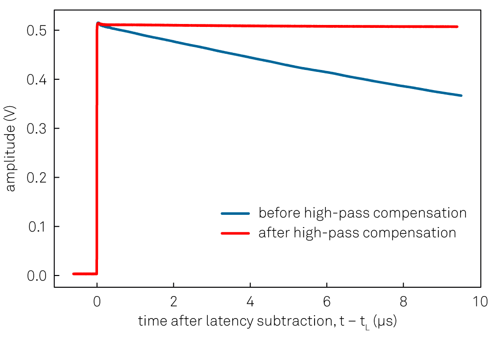
High-pass Compensation
The purpose of the high-pass compensation is to correct for first-order
high-pass filters such as DC blocks or bias-tees. An example of its
application is shown in Figure 3.The
only parameter of the high-pass compensation filter is the time constant
in units of seconds. When enabled, the high-pass compensation filter
introduces a delay of 12 clock cycles, which corresponds to 12/(300 MHz)
= 40 ns. Since the high-pass compensation filter integrates the signal
over time, it may be necessary to clear the filter regularly using the
AWG sequencer instruction setPrecompClear(1). Whenever this command is
placed in front of a playWave or playWaveDIO command, a clearing
signal is sent to the high-pass compensation filter synchronous to the
playWave or playWaveDIO command. The Clearing drop-down selector
defines when the clearing signal is sent relative to the waveform
playback: during the entire waveform playback (Level), at the start
(Rise), at the end (Fall), or both at the start and at the end (Both).
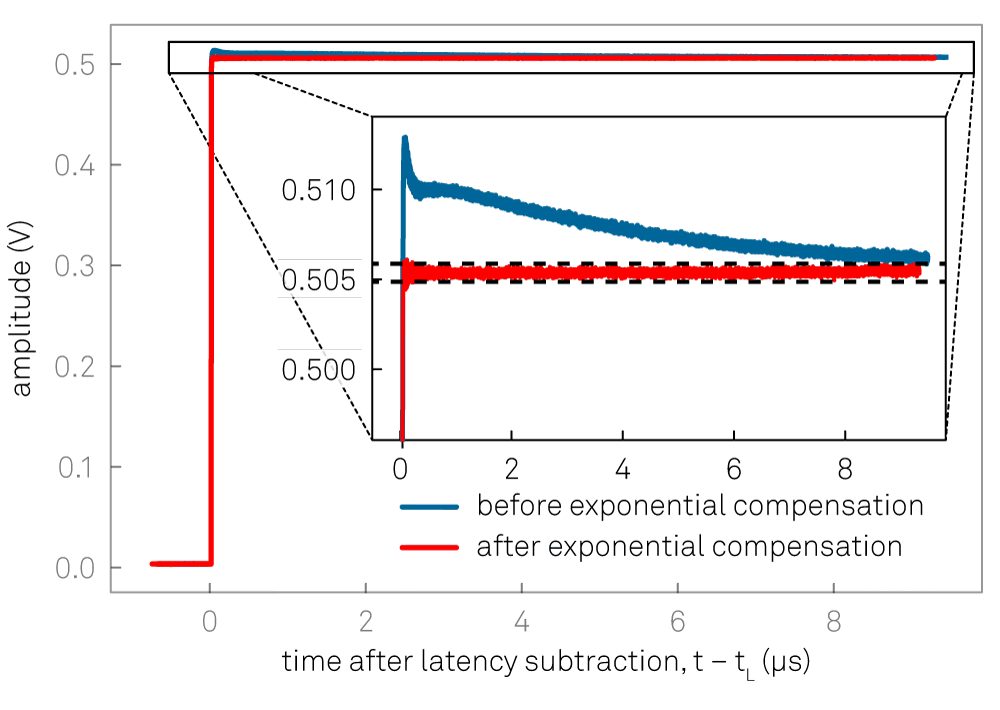
Exponential Compensation
The exponential overshoot and undershoot compensation filters can correct for exponential signal components typically introduced by spurious capacitances or inductances combined with resistors. An example of their application is shown in Figure 4. The parameters are the time constant of the exponential decay and the amplitude of the exponential relative to the input step size. A positive amplitude corrects for overshoots, while a negative amplitude corrects for undershoots. When enabled, each exponential compensation filter introduces a delay of 11 clock cycles, corresponding to 11/(300 MHz) = 36.67 ns.
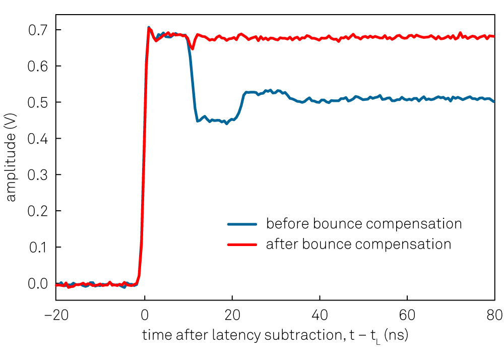
Bounce Compensation
The bounce compensation can be used to suppress unwanted reflections in the cables of the experimental setup. An example of its application is shown in Figure 5. The bounce compensation adds to the original input signal the input signal multiplied with a configurable relative amplitude and delay. When enabled, the bounce compensation filter introduces a delay of 4 clock cycles, corresponding to 13.33 ns.
Finite Impulse Response Filter
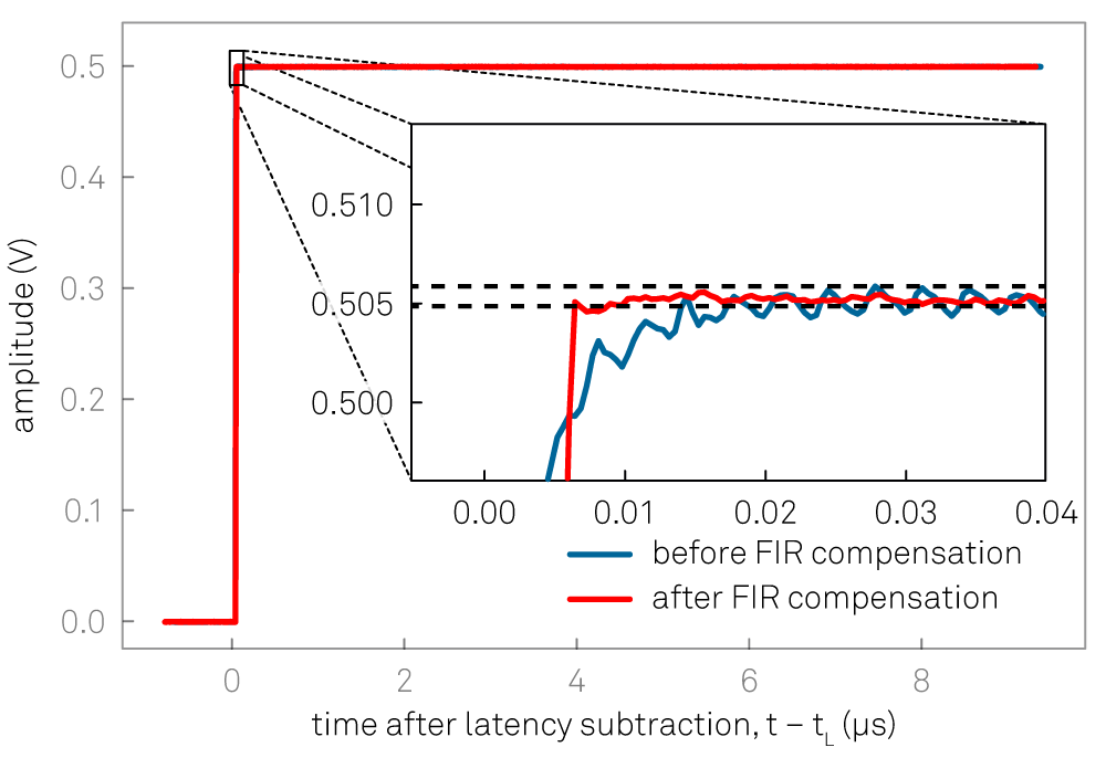
The real-time finite impulse response (FIR) filter is suitable for correcting signal transients on the nanosecond time scale. An example of its application is shown in Figure 6. The user can set 40 coefficients of the FIR filter kernel represented in the Device FIR sub-tab. The operation of the FIR filter corresponds to a convolution of the input signal with the FIR filter kernel. The first 8 coefficients are directly applied to the first eight taps of the FIR filter at the full time resolution. The remaining 32 coefficients are applied to pairs of taps. Therefore, the total number of taps is 8+2*32 = 72 and the user can choose 8+32 = 40 coefficients. The Device FIR sub-tab gives access to the coefficients from the graphical UI, which is suitable for quick manual tests. For systematic configuration of this filter, the use of the API is recommended.
Specification Table
| Parameter | Value |
|---|---|
| Number of precompensation units | 1 per AWG channel (4 or 8 total depending on HDAWG model) |
| Compensation filters per unit | 1× high-pass, 8× exponential, 1× bounce, 1× FIR |
| High-pass compensation filter type | IIR, configurable time constant |
| High-pass compensation time constant range | 208 ps to 166 ms |
| Exponential compensation filter type | IIR, configurable time constant and amplitude |
| Exponential compensation time constant range | 15 ns to 1 ms (available range depends on amplitude setting) |
| Bounce compensation filter type | FIR, configurable delay and amplitude |
| Bounce compensation delay range | 0 to 100 ns |
| Bounce compensation delay resolution | 1 sample period (417 ps at 2.4 GSa/s) |
| Bounce compensation amplitude range | -1 to +1 (dimensionless) |
| FIR filter type | Causal FIR filter, 72 coefficients (corresponding to 30 ns at 2.4 GSa/s), first 8 coefficients freely configurable,remaining 64 coefficients pairwise equal |
| FIR filter coefficients range | -4 to +4 (dimensionless) |
| FIR filter coefficients resolution | 18 bit |
| Precompensation Simulator display options | Forward filter, inverse filter, uncompensated step response |
Functional Elements
| Control/Tool | Option/Range | Description |
|---|---|---|
| Enable | ON / OFF | Enables the entire precompensation filter chain. |
| Total Latency | The total latency introduced by the entire precompensation filter chain. | |
| Status Flag Reset | Resets the status flags of all precompensation filters of this output channel. | |
| Enable | ON / OFF | Enables the exponential compensation filter. |
| Time Constant | Sets the characteristic time constant of the exponential compensation filter. | |
| Amplitude | Sets the amplitude of the exponential compensation filter relative to the signal amplitude. | |
| Status | Indicates the status of the exponential compensation filter: Green: normal, Red: overflow during the last update period (~100 ms), yellow: overflow occurred in the past. | |
| Enable | ON / OFF | Enables the high-pass compensation filter. |
| Time Constant | Sets the characteristic time constant of the high-pass compensation filter. | |
| Clearing Slope | Select when to react to a clearing pulse generated after the AWG Sequencer setPrecompClear instruction. | |
| Level | During the entire clearing pulse. | |
| Rise | At the beginning of the clearing pulse. | |
| Fall | At the end of the clearing pulse. | |
| Both | Both at the beginning and at the end of the clearing pulse. | |
| Status | Indicates the status of the high-pass compensation filter. Green: normal, Red: overflow during the last update period (~100 ms), yellow: overflow occurred in the past. | |
| Enable | ON / OFF | Enables the bounce correction filter. |
| Delay | Sets the delay of the bounce correction filter. | |
| Amplitude | Sets the amplitude of the bounce correction filter relative to the signal amplitude. | |
| Status | Indicates the status of the bounce correction filter: Green: normal, Red: overflow during the last update period (~100 ms), yellow: overflow occurred in the past. | |
| Enable | ON / OFF | Enables the finite impulse response (FIR) precompensation filter. |
| FIR Coefficient | FIR (finite impulse response) filter coefficients. The first 8 coefficients are applied to 8 individual samples, whereas the following 32 Coefficients are applied to two consecutive samples each. | |
| Status | Indicates the status of the finite impulse response (FIR) precompensation filter: Green: normal, Red: overflow during the last update period (~100 ms), yellow: overflowed in the past. | |
| Latency Simulation | Enables the simulation of the latency of the precompensated signal. | |
| Number of Points | Length of the simulated wave in number of sample points. | |
| Input Wave | Wave input source for the simulation. | |
| Step | Step function. | |
| Pulse | Single pulse. | |
| AWG Loading | Load an AWG sequencer wave from the AWG as specified with the AWG wave index. To apply the latest waveform, the corresponding AWG sequencer must be turned off. | |
| File | Load a wave from a CSV file as specified by the file selector. | |
| Open Directory | Opens the directory where the CSV files are expected to be located. This is OS specific and could open additional windows. | |
| Wave File (CSV) | Select the wave input file from the list of CSV files available in the Precompensation directory which can be accessed by pressing the Open Directory icon. | |
| Columns | The number of columns determined from the CSV file. | |
| Timestamp Column | The index of the column in the CSV file containing the timestamp for each sample. | |
| Data Column | The index of the column in the CSV file containing the samples. | |
| Sampling Frequency | The sampling frequency determined by the timestamps from the CSV file. | |
| Sample Delay | Artificial time delay of the simulation input. | |
| Gain | Artificial gain with which to scale the samples of the simulation input. | |
| Offset | Artificial vertical offset added to the simulation input. | |
| Status | The status of loading the CSV file. | |
| To Device | Copy the Simulation Filter parameters onto the respective Device Filter parameters. | |
| AWG Wave Index | Determines which AWG wave is loaded from the the AWG output. Internally, all AWG sequencer waves are indexed and stored. With this specifier, the respective AWG wave is loaded into the Simulation. | |
| To Simulator | Copy the Device Filter parameters onto the respective Simulation Filter parameters. |