Basic Waveform Playback¶

Note

This tutorial is applicable to all HDAWG Instruments.

Goals and Requirements¶

The goal of this tutorial is to demonstrate the basic use of the HDAWG. We demonstrate waveform generation and playback, triggering and synchronization. In order to visualize the multi-channel signals, an oscilloscope with sufficient bandwidth and channel number is required.

Preparation¶

Connect the cables as illustrated below. Make sure that the instrument is powered on and connected by Ethernet to your local area network (LAN) where the host computer resides. After starting LabOne, the default web browser opens with the LabOne graphical user interface.

Note

The instrument can also be connected via the USB interface, which can be simpler for a first test. As a final configuration for measurements, it is recommended to use the 1GbE interface, as it offers larger bandwidth.

Figure 1: Connections for the arbitrary waveform generator basic playback tutorial

The tutorial can be started with the default instrument configuration (e.g. after a power cycle) and the default user interface settings (e.g. as is after pressing F5 in the browser).

Waveform Generation and Playback¶

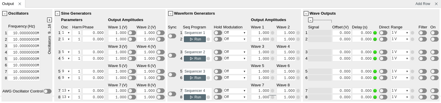
In this tutorial we generate signals with the AWG and visualize them with the scope. In a first step we enable the Wave outputs, but disable all sinusoidal signals generated by the sine generators by default. We also configure the scope with a suitable time base (e.g. 500 ns per division) and range (e.g. 0.2 V per division) The following table summarizes the necessary settings.

Table 1: Settings: enable the output
Tab	Section	#	Label	Setting / Value / State
Output	Wave Outputs	1	Enable	ON
Output	Wave Outputs	2	Enable	ON
Output	Sine Generators	1&2	Wave 1 Enable	OFF
Output	Sine Generators	1&2	Wave 2 Enable	OFF

Table 2: Settings: configure the external scope
Scope Setting	Value / State
Ch1 enable	ON
Ch1 range	0.2 V/div
Timebase	500 ns/div
Trigger source	Ch1
Trigger level	100 mV
Run / Stop	ON

In the Output tab, we configure the first output channel. The final signal amplitude is given by the product of the full scale output range of 1 V, the dimensionless amplitude scaling factor 1.0, and the actual dimensionless signal amplitude stored in the waveform memory. The necessary settings are summarized in the following table.

Table 3: Settings: configure the AWG output
Tab	Sub-tab	Section	#	Label	Setting / Value / State
Seq	Control			Sampling Rate	2.4 GHz
Output		Waveform Generators	1	Amplitude	1.0
Output		Waveform Generators	1	Modulation	OFF
Output		Wave Outputs	1	Range	1 V
Output		Wave Outputs	1	Enable	ON

To operate the AWG we need to specify a sequence program. This can be done interactively by typing the program in the Sequence window. Let’s start by typing the following code into the sequence editor.

wave w_gauss = 1.0*gauss(8000, 4000, 1000);
playWave(1, w_gauss);

In the first line of the program, we generate a waveform with a Gaussian shape with a length of 8000 samples and store the waveform under the name w_gauss. The peak center position 4000 and the standard deviation 1000 are both defined in units of samples. You can convert them into time by dividing by the chosen Rate (2.4 GSa/s by default). The waveform generated by the gauss function has a peak amplitude of 1. This amplitude is dimensionless and the physical signal amplitude is given by this number multiplied with the Wave output range (here we chose 1.0 V). We put a scaling factor of 1.0 in place which can be replaced by any other value. The code line is terminated by a semicolon according to C conventions. With the second line of the program, the generated waveform w_gauss is played on AWG Output 1.

Note

For this tutorial, we will keep the description of the Sequencer instructions short. You can find the full specification of the LabOne Sequencer language in LabOne Sequence Programming

Note

The AWG has a waveform granularity of 16 samples. It’s recommended to use waveform lengths that are multiples of 16, e.g. 8000 like in this example, to avoid having ill-defined samples between successively played waveforms. Waveforms with other lengths are allowed, but they get padded with zeros by the compiler. This may be undesired in some cases, specifically when using the Hold feature of the AWG.

If we now click on , the program gets compiled. This means the program is translated into instructions for the LabOne Sequencer on the instrument, see AWG Sequencer Tab. If no error occurs (due to wrong program syntax, for example), the Compiler Status LED lights up green, and the resulting program as well as the waveform data is written to the instrument memory. If an error or warning occurs, messages in the Compiler Status field will help in debugging the program. If we now have a look at the Waveform sub-tab, we see that our Gaussian waveform appeared in the list. The Memory Usage field at the bottom of the Waveform sub-tab shows what fraction of the instrument memory is filled by the waveform data. The Waveform Viewer sub-tab allows you to graphically display the currently marked waveform in the list.

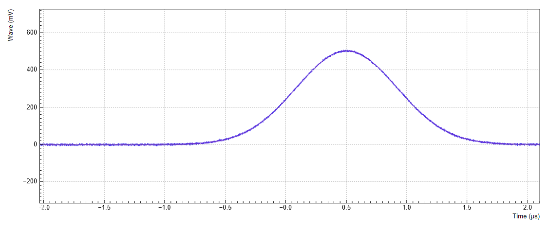
By clicking on , we have the AWG execute our program once. Since we have armed the scope previously with a suitable trigger level, it has captured our Gaussian pulse with a FWHM of about 1.0 μs as shown in Figure Figure 3.

Figure 3: Gaussian pulse as generated by the AWG and captured by the scope

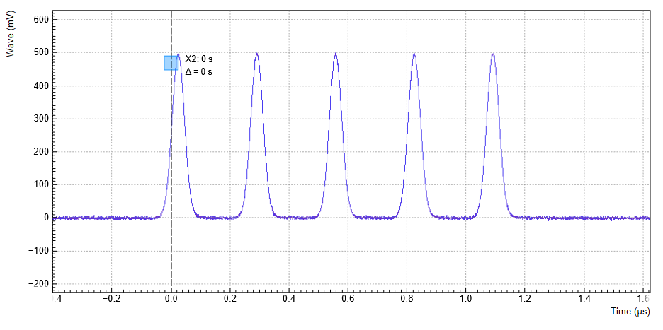
The LabOne Sequencer language offers a lot of run-time control. The basic functionality is to repeat a waveform several times. In the following example, all the code within the curly brackets {...} is repeated 5 times. Upon clicking and , you should observe 5 short Gaussian pulses in a new scope shot, see Figure 4.

wave w_gauss = 1.0 * gauss(640, 320, 50);

repeat (5) {
  playWave(1, w_gauss);
}

Figure 4: Burst of Gaussian pulses generated by the AWG and captured by the scope

In order to generate more complex waveforms, the LabOne Sequencer programming language offers a rich toolset for waveform editing. On the basis of a selection of standard waveform generation functions, waveforms can be added, multiplied, scaled, concatenated, and truncated. It’s also possible to use compile-time evaluated loops to generate pulse series with systematic parameter variations – see LabOne Sequence Programming for more precise information. In the following code example, we make use of these tools to generate a pulse with a smooth rising edge, a flat plateau, and a smooth falling edge. We use the cut function to cut a waveform at defined sample indices, the rect function to generate a waveform with constant level 1.0 and length 320, and the join function to concatenate three (or arbitrarily many) waveforms.

wave w_gauss = gauss(640, 320, 50);
wave w_rise = cut(w_gauss, 0, 319);
wave w_fall = cut(w_gauss, 320, 639);
wave w_flat = rect(320, 1.0);

wave w_pulse = join(w_rise, w_flat, w_fall);

while (true) {
  playWave(1, w_pulse);
}

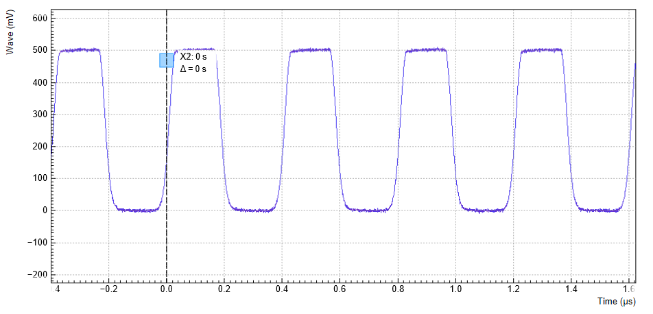
Note that we replaced the finite repetition by an infinite repetition by using a while loop. Loops can be nested in order to generate complex playback routines. The output generated by the program above is shown in Figure 5.

Figure 5: Infinite pulse series generated by the AWG and captured by the scope

As programs get longer, it becomes useful to store and recall them. Clicking on allows you to store the present program under a new name. Clicking on then saves your program to the file name displayed at the top of the editor. As you begin to work on sequence programs more regularly, it’s worth expanding your repertoire using some of the editor keyboard shortcuts listed in Sequence Editor Keyboard Shortcuts.

It’s also possible to iterate over the samples of a waveform array and calculate each one of them in a loop over a compile-time variable cvar. This often allows to go beyond the possibilities of using the predefined waveform generation function, particularly when using nested formulas of elementary functions like in the following example. The waveform array needs to be pre-allocated e.g. using the instruction zeros.

const N = 1024;
const width = 100;
const position = N/2;
const f_start = 0.1;
const f_stop = 0.2;
cvar i;
wave w_array = zeros(N);
for (i = 0; i < N; i++) {
  w_array[i] = sin(10/(cosh((i-position)/width)));
}

playWave(w_array);

Should you require more customization than what is offered by the LabOne AWG Sequencer language, it’s possible to load a waveform directly from the API. In the sequence the waveform should be declared using the placeholder function to define size and type of the waveform.

const LENGTH = 1024;
wave w = placeholder(LENGTH, true, false); // Create a waveform of size LENGTH, with one marker
assignWaveIndex(1, w, 10);                 // Create a wave table entry with placeholder waveform
                                           // routed to output 1, with index 10
playWave(1, w);

This sequence will not run until a valid waveform has been loaded. This can be done for example in Python using the Zurich Instruments Toolkit:

## Load the LabOne API and other necessary packages
from zhinst.toolkit import Session
from zhinst.toolkit import Waveforms
import numpy as np

device_id='dev8000'
server_host = 'localhost'

### connect to data server
session = Session(server_host)
### connect to device
device = session.connect_device(device_id)

##Generate a waveform and marker
LENGTH = 1024
wave = np.sin(np.linspace(0, 10*np.pi, LENGTH))*np.exp(np.linspace(0, -5, LENGTH))
marker = np.concatenate([np.ones(32), np.zeros(LENGTH-32)]).astype(int)

## Upload waveforms
AWG_INDEX = 0 #use AWG 1
waveforms = Waveforms()
waveforms[10] = (wave,None,marker) # I-component wave, Q-component None, marker
device.awgs[AWG_INDEX].write_to_waveform_memory(waveforms)

The waveform data can be arbitrary, but consider that the final signal will pass through the output stage of the instrument. This means that signal components exceeding the output stage bandwidth are not reproduced exactly as suggested for example by looking at a plot of the waveform data. In particular, this concerns sharp transitions from one sample to the next.

In the usage of the instructions 'placeholder', 'assignWaveIndex', and 'playWave', there are a number of caveats due to the implicit creation of waveform table entries depending on the output channel assignment (the optional first arguments of 'assignWaveIndex' and 'playWave' instructions). The following code is for example valid, but not recommended because it is poorly readable:

const LENGTH = 1024;
wave w = placeholder(LENGTH);
assignWaveIndex(1, w, 10);
assignWaveIndex(w, w, 11);

playWave(1, w);
playWave(w, w);

Instead, it’s recommended to use a unique waveform variable name for each intended single-channel memory entry, and to use this variable name with consistent output channel assignment in 'placeholder', 'assignWaveIndex', and 'playWave' as is done in the following example:

const LENGTH = 1024;
wave w_a = placeholder(LENGTH, true, true);
wave w_b = placeholder(LENGTH, true, true);
wave w_c = placeholder(LENGTH, true, true);
assignWaveIndex(1, w_a,   10);
assignWaveIndex(w_b, w_c, 11);

playWave(1, w_a);
playWave(w_b, w_c);

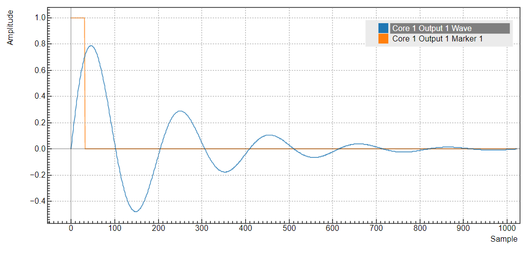
In the latter case, a possible Python code to update the wave table is shown below. Note that we use the full amount of markers available in this example. The marker integer array encodes the available markers in its least significant bits. When uploading 2 or more waveforms like in this example, it is recommended to perform the waveform upload with a single set command. This is possible by combining multiple pairs of waveform addresses and data as a Python list of tuples, and using this list as the argument of the set command. In this way, the overhead in communication latency is paid only once, and waveform upload is much faster than when issuing a set command for each waveform.

Note

The set command is only available with the Python API. Other APIs are limited to the use of setVector. setVector does not support combining multiple commands into one. Apart from that, its usage is identical to that of set.

## Load the LabOne API and other necessary packages
from zhinst.toolkit import Session
from zhinst.toolkit import Waveforms
import numpy as np

DEVICE_ID = 'DEVXXXX'
SERVER_HOST = 'localhost'

session = Session(SERVER_HOST)              ## connect to data server
device = session.connect_device(DEVICE_ID)  ## connect to device

##Generate a waveform and marker
LENGTH = 1024
wave_a = np.sin(np.linspace(0, 10*np.pi, LENGTH))*np.exp(np.linspace(0, -5, LENGTH))
wave_b = np.sin(np.linspace(0, 20*np.pi, LENGTH))*np.exp(np.linspace(0, -5, LENGTH))
wave_c = np.sin(np.linspace(0, 30*np.pi, LENGTH))*np.exp(np.linspace(0, -5, LENGTH))

marker_a  = np.concatenate([  0b11*np.ones(32), np.zeros(LENGTH-32)]).astype(int)
marker_bc = np.concatenate([0b1111*np.ones(32), np.zeros(LENGTH-32)]).astype(int)

##Convert and send them to the instrument
AWG_INDEX = 0 #use AWG 1
waveforms = Waveforms()
waveforms[10] = (wave_a,None,marker_a)
waveforms[11] = (wave_b,wave_c,marker_bc)
device.awgs[AWG_INDEX].write_to_waveform_memory(waveforms)

In channel grouping modes, see Multi-Channel Playback , 2x4 or 1x8 (1x4 in HDAWG-4) the usage of 'placeholder', 'assignWaveIndex' combined with 'playWave' is also supported. However, in these modes it is more difficult to infer the format and content of the wave tables on the separate AWG cores from the high-level sequence program. When possible, use the default grouping mode 4x2 (2x2 in HDAWG-4). In other modes, follow the same basic guideline of using unique waveform variable names and consistent use of 'assignWaveIndex' and 'playWave' instructions. As an example, to create dual-channel waveform table entries on the AWG cores 1 and 2, group at least 4 channels together by choosing the 2x4 (1x4 in HDAWG-4) mode. Both entries have the index 10 and need to be filled with data separately using the respective API nodes 'device.awgs[0].waveform.waves[10]' and 'device.awgs[1].waveform.waves[10]'.

const LENGTH = 1024;
wave w_a = placeholder(LENGTH, true, true);
wave w_b = placeholder(LENGTH, true, true);
wave w_c = placeholder(LENGTH, true, true);
wave w_d = placeholder(LENGTH, true, true);

assignWaveIndex(w_a, w_b, w_c, w_d, 10);

playWave(w_a, w_b, w_c, w_d);

Python code to fill the wave table in this case is shown below.

## Load the LabOne API and other necessary packages
from zhinst.toolkit import Session
from zhinst.toolkit import Waveforms
import numpy as np

DEVICE_ID = 'DEVXXXX'
SERVER_HOST = 'localhost'

session = Session(SERVER_HOST)              ## connect to data server
device = session.connect_device(DEVICE_ID)  ## connect to device

##Generate a waveform and marker
LENGTH = 1024
wave_a = np.sin(np.linspace(0, 10*np.pi, LENGTH))*np.exp(np.linspace(0, -5, LENGTH))
wave_b = np.sin(np.linspace(0, 20*np.pi, LENGTH))*np.exp(np.linspace(0, -5, LENGTH))
wave_c = np.sin(np.linspace(0, 30*np.pi, LENGTH))*np.exp(np.linspace(0, -5, LENGTH))
wave_d = np.sin(np.linspace(0, 40*np.pi, LENGTH))*np.exp(np.linspace(0, -5, LENGTH))

marker_ab = np.concatenate([0b1111*np.ones(32), np.zeros(LENGTH-32)]).astype(int)
marker_cd = np.concatenate([0b1111*np.ones(32), np.zeros(LENGTH-32)]).astype(int)

## Define waveforms
waveforms_0 = Waveforms() #waveforms for AWG 1
waveforms_1 = Waveforms() #waveforms for AWG 2
waveforms_0[10] = (wave_a,wave_b,marker_ab)
waveforms_1[10] = (wave_c,wave_d,marker_cd)
## Send to instrument
with device.set_transaction():
    device.awgs[0].write_to_waveform_memory(waveforms_0)
    device.awgs[1].write_to_waveform_memory(waveforms_1)

Alternatively to the waveform upload via an API, you can import any waveform from a file. If the file is stored in the location (C:\Users\<user name>\Documents\Zurich Instruments\LabOne\WebServer\awg\waves\ under Windows or ~/Zurich Instruments/LabOne/WebServer/awg/waves/ under Linux), you can then play back the wave by referring to the file name without extension in the sequence program:

playWave("wave_file");

If you prefer, you can also store it in a wave data type first and give it a new name:

wave w = "wave_file";
playWave(w);

For more information about the file format, please refer to the LabOne Programming Manual, section AWG Module.

Triggering and Synchronization¶

Now we have a look at the triggering functionality of the AWG. In this section you will learn about the most important use cases: - Triggering the AWG with an external TTL signal - Generating a TTL signal with the AWG to trigger another piece of equipment

Triggering the AWG¶

In this section we show how to trigger the AWG with an external TTL signal. We start by generating a periodic TTL signal using the external scope (on the trigger, sync, or auxiliary output), if it has this capability, or by using another source of such a signal, e.g., a function generator. Generate a signal with the parameters listed in the following table.

Table 4: Settings: generate a 300 kHz TTL signal
Setting	Value / State
Signal type	square wave
Signal level	0 V / 3.3 V
Frequency	300 kHz

We then connect this square signal to the HDAWG Trig input 1, and separately monitor the signal on the scope using a power splitter or a T-piece. The figure below shows the connection used.

Figure 7: Connections for triggering the arbitrary waveform generator

The AWG internally has 2 digital trigger input channels. These are not directly associated with physical device inputs but can be freely configured to probe a variety of internal or external signals. Here, we link the AWG Digital Trigger 1 to the physical Trig 1 connector.

Table 5: Settings: configure the AWG analog trigger input
Tab	Sub-tab	Section	#	Label	Setting / Value / State
Seq	Trigger	Digital Trigger 1		Signal	Trigger In 1
Seq	Trigger	Digital Trigger 1		Slope	Rise

Finally, we modify our last AWG program by including a waitDigTrigger instruction just before the playWave instruction. The result is that upon every repetition inside the infinite while loop, the AWG will wait for a rising edge on Trigger input 1.

wave w_gauss = gauss(640, 320, 50);
wave w_rise  = cut(w_gauss, 0, 319);
wave w_fall  = cut(w_gauss, 320, 639);
wave w_flat  = rect(320, 1.0);

wave w_pulse = join(w_rise, w_flat, w_fall);

while (true) {
  waitDigTrigger(1);
  playWave(1, w_pulse);
}

Compile and run the above program. Figure 8 shows the pulse series as seen in the scope: the pulses are now spaced by the oscillator period of about 3.3 μs, unlike previously when the period was determined by the length of the waveform w_pulse. Try changing the trigger signal frequency or unplugging the trigger cable to observe the immediate effect on the signal.

Figure 8: Externally triggered pulse series generated by the AWG and captured by the scope. The AWG signal is shown in blue, the external trigger signal (attenuated by 20 dB) is shown in green.

Generating Trigger and Marker Outputs with the AWG¶

There are two ways of generating trigger output signals on the Mark Channel: with digital marker bits, or through sequencer instructions.

The method using digital marker bits is recommended when precise timing is required and/or complicated serial bit patterns need to be played on the Mark front panel output. Digital marker bits are part of the data of every waveform, which is an array of 18-bit words: 16 bits of each word represent the analog waveform data, and the remaining 2 are digital marker bits. A digital marker bit is assigned to the Mark front panel output, and upon playing the waveform, a sample-precise trigger signal is generated based on the value of the digital marker bit.

The method using a sequencer instruction is simpler, but the timing control is less powerful than when using markers. It is useful for instance to generate a single trigger signal at the start of an AWG program.

Table 6: Comparison: AWG markers and triggers
	Marker	Trigger
Implementation	Part of waveform	Sequencer instruction
Timing control	High	Low
Generation of serial bit patterns	Yes	No
Cross-device synchronization	Yes	Yes

Let us first demonstrate the use of markers . In the following code example we first generate a Gaussian pulse again. The generated wave actually does include marker bits – they are simply set to zero by default. We use the marker function to assign the desired non-zero marker bits to the wave. The marker function takes two arguments, the first is the length of the wave, the second is the marker configuration in binary encoding: the value 0 stands for a both marker bits low, the values 1, 2, and 3 stand for the first, the second, and both marker bits high, respectively. We use this to construct the wave called w_marker.

const marker_pos = 3000;

wave w_gauss  = gauss(8000, 4000, 1000);
wave w_left   = marker(marker_pos, 0);
wave w_right  = marker(8000-marker_pos, 1);
wave w_marker = join(w_left, w_right);
wave w_gauss_marker = w_gauss + w_marker;

playWave(1, w_gauss_marker);

The waveform addition with the '+' operator adds up analog waveform data but also combines marker data. The wave w_gauss contains zero marker data, whereas the wave w_marker contains zero analog data. Consequently the wave called w_gauss_marker contains the merged analog and marker data. We use the integer constant marker_pos to determine the point where the first marker bit flips from 0 to 1 somewhere in the middle of the Gaussian pulse.

Note

The add function and the '+' operator combine marker bits by a logical OR operation. This means combining 0 and 1 yields 1, and combining 1 and 1 yields 1 as well.

There is a certain freedom to assign different marker bits to different Mark outputs. The following table summarizes the settings to apply in order to output marker bit 1 on Mark 1.

Table 7: Settings: configure the AWG marker output and scope trigger
Tab	Sub-tab	Section	#	Label	Setting / Value / State
DIO		Marker Out	2	Signal	Output 1 Marker 1
DIO		Output	2	Drive	ON
Scope	Trigger	Trigger		Signal	Trig Input 1

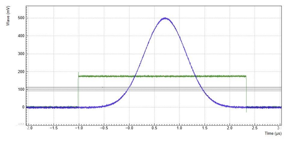
We connect the Mark 1 signal to one of the scope channels as shown below.

Figure 9: Connections for generating marker signals with the arbitrary waveform generator

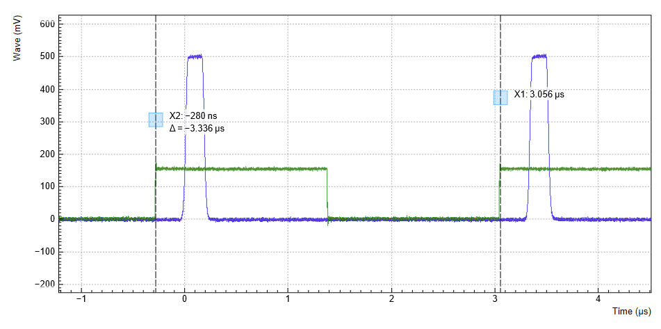
Figure 10 shows the AWG signal captured by the scope as a blue curve. The green curve shows the second scope channel displaying the marker signal. Try changing the marker_pos constant and re-running the sequence program to observe the effect on the temporal alignment of the Gaussian pulse.

Figure 10: Gaussian pulse and square marker signal generated by the AWG and captured by the scope

Let us now demonstrate the use of sequencer instructions to generate a trigger signal. Copy and paste the following code example into the Sequence Editor.

wave w_gauss = gauss(8000, 4000, 1000);

setTrigger(1);
playWave(1, w_gauss);
waitWave();
setTrigger(0);

The setTrigger function takes a single argument encoding the four trigger output states in binary manner – the integer number 1 corresponds to a configuration of 0/0/0/1 for the trigger outputs 4/3/2/1. The binary integer notation of the form 0b0000 is useful for this purpose – e.g. setTrigger(0b0011) will set trigger outputs 1 and 2 to 1, and trigger outputs 3 and 4 to 0. We included a waitWave instruction after the playWave instruction. It ensures that the subsequent setTrigger instruction is executed only after the Gaussian wave has finished playing, and not during waveform playback.

Note

The 'waitWave' instruction represents a means to control the timing of instructions in the the Wait & Set and the Playback queue which are described in the section AWG Architecture and Execution Timing. In the example above, the waitWave instruction puts the playback of the next instruction in the Wait & Set queue, the setTrigger(0), on hold until the waveform is finished. Without the 'waitWave' instruction, the AWG trigger would return to zero at the beginning of the waveform playback.

Note

Between consecutive 'playWave' and 'playZero' instructions, the use of 'waitWave' is explicitly not required. Sequential instructions in the playback queue are played immediately after one another, back to back.

We reconfigure the Mark 1 connector in the DIO tab such that it outputs 'AWG Trigger 1', instead of 'Output 1 Marker 1'. The rest of the settings can stay unchanged.

Table 8: Settings: configure the AWG trigger output
Tab	Sub-tab	Section	#	Label	Setting / Value / State
DIO		Marker Out	1	Signal	AWG Trigger 1

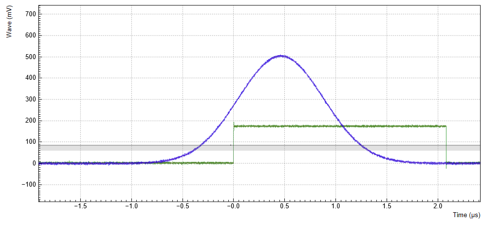
Figure 11 shows the AWG signal captured by the scope. This looks very similar to Figure 10 in fact. With this method, we’re less flexible in choosing the trigger time, as the rising trigger edge will always be at the beginning of the waveform. But we don’t have to bother about assigning the marker bits to the waveform.