Simple Loop
Note
This tutorial is applicable to all MFLI Instruments. No specific options are required.
Goals and Requirements
This tutorial is for people with no or little prior experience with Zurich Instruments lock-in amplifiers. By using a very basic measurement setup, this tutorial shows the most fundamental working principles of the MFLI Instrument and the LabOne UI in a step-by-step hands-on approach.
There are no special requirements for this tutorial.
Preparation
In this tutorial, you are asked to generate a single-ended signal with the MFLI Instrument and measure that generated signal with the same instrument using an internal reference. This is done by connecting Signal Output +V to Signal Input +V with a short BNC cable (ideally < 30 cm). Alternatively, it is possible to connect the generated signal at Signal Output +V to an oscilloscope by using a T-piece and an additional BNC cable. Figure 1 displays a sketch of the hardware setup.

Note
This tutorial is for all MFLI irrespective of which particular option set is installed. Some changes in the description apply if the MF-MD Multi-demodulator option is installed.
Connect the cables as described above. Make sure that the MFLI Instrument is powered on and then connect the MFLI directly by USB to your host computer or by Ethernet to your local area network (LAN) where the host computer resides. After connecting to your Instrument through the web browser using its address, the LabOne graphical user interface is opened. Check the Getting Started for detailed instructions. The tutorial can be started with the default instrument configuration (e.g. after a power cycle) and the default user interface settings (i.e. as is after pressing F5 in the browser).
Generate the Test Signal
Perform the following steps in order to generate a 300 kHz signal of 0.5 V peak amplitude on Signal Output +V. We work with the graphical Lock-in tab. Note that the control elements in this tab dynamically adapt their appearance to the web browser window size. Be sure to work in full screen size for this test.
-
In the Lock-in tab, select the sub-tab 1 on the left-hand side of the screen. In the Reference section, change the frequency value of oscillator 1 to 300 kHz: click on the field, enter 300000 or 300 k in short and press either Tab or Enter on your keyboard to activate the setting.
-
In the Output Amplitudes section, set the amplitude to 500 mV (peak value) and enable the signal by clicking on the button labeled "En". A single green LED on top indicates the enabled signal.
-
In the Signal Output 1 section (right hand side on the Lock-in tab), set the Range pull-down to 1 V and the Offset to 0 V. Keep the Add and Diff buttons unchecked.
-
By default, all physical outputs of the MFLI are inactive to prevent damage to the MFLI or to the devices connected to it. Now it is time to turn on the main output by clicking on the button labelled "On".
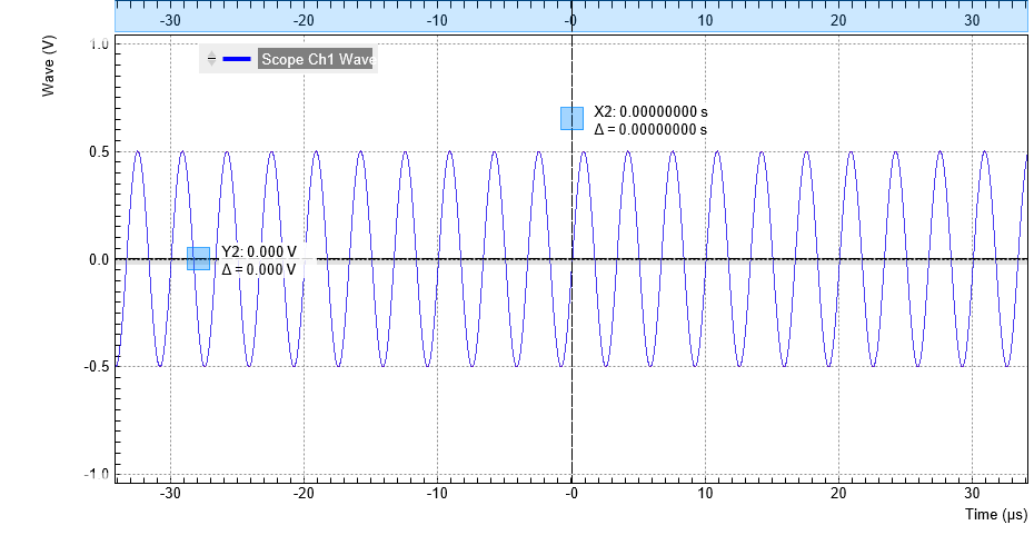
Table 1 summarizes the instrument settings to be made. If you have an oscilloscope connected to the setup, you should now be able to see the generated sinusoidal signal with a peak-to-peak amplitude of 1 V. Be sure to choose a high input impedance on the oscilloscope. But you can easily spare the extra equipment, as the MFLI comes with a built-in oscilloscope. In Check the Test Input Signal we describe how to use it.
| Tab | Section | # | Label | Setting / Value / State |
|---|---|---|---|---|
| Lock-in | Oscillator | 1 | Frequency | 300 kHz |
| Lock-in | Output | 1 | Amplitude | 500 mV |
| Lock-in | Output | 1 | Offset | 0 V |
| Lock-in | Output | 1 | On | On |
Check the Test Input Signal
Next, we configure the signal input side of the MFLI from the Lock-in tab, and then visualize the input signal using the Scope tab. In the Signal Input section of the Lock-in tab, select Sig In 1 from the pull-down menu. Set the range to 1.0 V, and be sure to have the AC, 50 Ω, Diff and Float buttons unchecked.
The range setting ensures that the analog amplification on the Signal Input +V is set such that the resolution of the input analog-to-digital converter is used efficiently without clipping the signal. This optimizes the dynamic range.
The incoming signal can now be observed over time by using the Scope tab. A Scope view can be placed in the web browser by clicking on the icon in the left sidebar or by dragging the Scope Icon to one of the open tab rows. Choose the following settings on the Scope tab to display the signal entering Signal Input +V:
| Tab | Section | # | Label | Setting / Value / State |
|---|---|---|---|---|
| Lock-in | Signal Input | 1 | Float | Off |
| Lock-in | Signal Input | 1 | Diff | Off |
| Lock-in | Signal Input | 1 | 50 Ω | Off |
| Lock-in | Signal Input | 1 | AC | Off |
| Scope | Horizontal | Sampling Rate | 60 MHz | |
| Scope | Horizontal | Length | 4096 pts | |
| Scope | Vertical | Channel 1 | Signal Input 1 | |
| Scope | Trigger | Enable | On | |
| Scope | Trigger | Level | 0 V |
The Scope tool now displays single shots of Signal Input +V with a temporal distance given by the Hold off Time. The scales on the top and on the left of the graphs indicate the zoom level for orientation. The icons on the left and below the figure give access to the main scaling properties and allow one to store the measurement data as a SVG image file or plain data text file. Moreover, panning can be achieved by clicking and holding the left mouse button inside the graph while moving the mouse.
Note
Zooming in and out along the horizontal dimension can by achieved with the mouse wheel. For vertical zooming, the shift key needs to be pressed and again the mouse wheel can by used for adjustments. Another, quick way of zooming in is to hold down the shift key and to use the left mouse button to define a horizontal, vertical, or box-like inside the graph area.
Having set the Input Range to 1 V ensures that no signal clipping occurs. If you set the Input Range to 0.1 V, clipping can be seen immediately on the scope window accompanied by a red OVI error flag on the status bar on the bottom of the LabOne User Interface. At the same time, the LED next to the Signal Input +V BNC connector on the instrument’s front panel will turn red.
The Scope is a very handy tool to quickly check the quality of the input signal and to adjust a suitable input range setting. For the full description of the Scope tool please refer to the Scope Tab.
Measure the Test Input Signal
Now, we are ready to use the MFLI to demodulate the input signal and measure its amplitude and phase. We will use two tools of the LabOne User Interface: the Numeric and the Plotter tab.
First, adjust the parameters listed in the following table on the graphical Lock-in tab for demodulator 1.
| Tab | Section | # | Label | Setting / Value / State |
|---|---|---|---|---|
| Lock-in | Signal Input | 1 | Signal Input 1 | |
| Lock-in | Low-Pass Filter | 1 | Sinc | Off |
| Lock-in | Low-Pass Filter | 1 | Order | 3 (18 dB/Oct) |
| Lock-in | Low-Pass Filter | 1 | BW 3 dB | 10.6 Hz |
| Lock-in | PC Data Transfer | 1 | En | On |
| Lock-in | PC Data Transfer | 1 | Rate | 100 Sa/s (automatically adjusted to 104.6 Sa/s) |
| Lock-in | PC Data Transfer | 1 | Trigger | Continuous |
These above settings configure the demodulation filter to the third-order low-pass operation with a 10.6 Hz 3 dB filter bandwidth (BW 3dB). Alternatively, the corresponding noise-equivalent bandwidth (BW NEP) or the integration time constant (TC) can be displayed and entered. The output of the demodulator filter is read out at a rate of 104.6 Hz, implying that 104.6 data samples are sent to the internal MFLI computer per second with equidistant spacing. These samples can be viewed in the Numeric and the Plotter tool which we will examine now.
Note
-
The rate should be about 7 to 10 times higher than the filter bandwidth chosen in the Low-Pass Filter section. When entering a number in the Rate field, the new rate is automatically set to the closest available value - in this case 104.6 Sa/s.
-
If you don’t see any signal in the Plotter, Numeric, Spectrum, DAQ, or Sweeper tab, the first thing to check is whether the corresponding data stream is enabled
The Numeric tool provides the space for 16 or more measurement panels. Each of the panels has the option to display the samples in the Cartesian (X,Y) or in the polar format (R,THETA) plus other quantities such as the Oscillator Frequencies and Auxiliary Inputs. The unit of the (X,Y,R) values are by default given in VRMS. The scaling and the displayed unit can be altered in the Signal Input section of the Lock-in tab. The numerical values are supported by graphical bar scale indicators to achieve better readability, e.g. for alignment procedures. Certain users may observe rapidly changing digits. This is due to the fact that you are measuring thermal noise that is maybe in the μV or even nV range depending on the filter settings. This provides a first glimpse of the level of measurement precision offered by your MFLI Instrument. If you wish to play around with the settings, you can now change the amplitude of the generated signal, and observe the effect on the demodulator output.
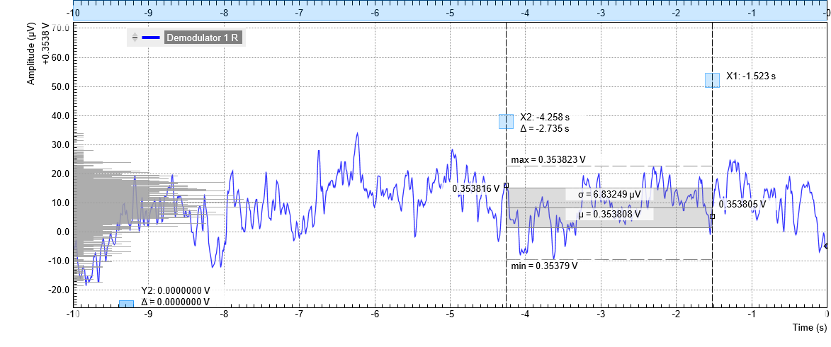
Next, we will have a look at the Plotter tool that allows users to observe the demodulator signals as a function of time. It is possible to adjust the scaling of the graph in both directions, or make detailed measurements with 2 cursors for each direction. You can find a variety of handy tools for immediate analysis in the Math sub-tab, allowing you to accurately measure noise amplitude, peak positions and heights, signal background and many more. Figure 3 shows the signal along with additional graphical elements that are dynamically added to the plot when e.g. using the histogram functionality from the Math sub-tab.
Signals of the same unit are automatically added to the same default y-axis group. This ensures that the axis scaling is identical. Signals can be moved between groups. More information on y-axis groups can be found in Plot Functionality. Try zooming in along the time dimension using the mouse wheel or the icons below the plot to display about one second of the data stream. While zooming in, the mode in which the data are displayed will change from a min-max envelope plot to linear point interpolation. The LabOne Web Server makes this choice depending on the density of points along the horizontal axis as compared to the number of pixels available on the screen.
Data displayed in the Plotter can also be saved continuously to the instrument memory and easily transferred to the host computer. Please have a look at Saving and Loading Data for a detailed description of the data saving and recording functionality. Instrument and user interface settings can be saved and loaded using the Config tab (Settings section).
Note
The MFLI is able to measure DC signals by setting the oscillator frequency to 0 Hz. The Demodulator R signal in this case differs by a factor of √2 from the actual DC voltage on the input, which needs to be taken into account. This may be systematically corrected by entering a scaling factor 0.7071 in the Signal Inputs section of the Lock-in tab.
Different Filter Settings
As next step in this tutorial you will learn to change the filter settings and see their effect on the measurement results. For this exercise, change the 3 dB bandwidth to 1 kHz.
| Tab | Section | # | Label | Setting / Value / State |
|---|---|---|---|---|
| Lock-in | Low-Pass Filter | 1 | Order | 3 (18 dB/Oct) |
| Lock-in | Low-Pass Filter | 1 | BW 3dB | 1 kHz |
| Lock-in | PC Data Transfer | 1 | Rate | 6.7 kSa/s |
Increasing the filter bandwidth reduces the integration time of the demodulators. This will increase available time resolution but in turn make the signal noisier, as can be nicely observed in the Plotter tab. Note that it is recommended to keep the sample rate 7 to 10 times the filter 3 dB bandwidth. The sample rate will be rounded off to the next available sampling frequency. For example, typing 7 k in the Rate field will result in 6.7 kSa/s which is sufficient to not only properly resolve the signal, but also to avoid aliasing effects.
Moreover, you may for instance "disturb" the demodulator with a change of test signal amplitude, for example from 0.5 V to 0.7 V and back. The plot will go out of the display range which can be re-adjusted by pressing the "Rescale" button
