Phase-locked Loop
Note
This tutorial is applicable to MF Instruments with the MF-PID Quad PID/PLL Controller option installed.
Goals and Requirements
This tutorial explains how to track the resonance frequency shift of a resonator using a phase-locked loop (PLL). To follow this tutorial, one needs to connect a resonator between Signal Output 1 and Signal Input 1.
Preparation
Connect the cables as shown in the figure below. Make sure that the MF Instrument is powered on and connected by USB to your host computer or by Ethernet to your local area network (LAN) where the host computer resides. After starting LabOne the default web browser opens with the LabOne graphical user interface.

The tutorial can be started with the default instrument configuration (e.g. after a power cycle) and the default user interface settings (e.g. as is after pressing F5 in the browser).
Determine the Resonance of the Quartz
In this section you will learn first how to find the resonance of your resonator with the Sweeper Tab tool. In the Sweeper tab, one can start by defining a frequency sweep across the full instrument bandwidth and narrow down the range using multiple sweeps in order to find the resonance peak of interest. In our case, we know already that the resonance lies at around 1.8 MHz which saves us some time in finding the peak, knowing that its Q factor is rather high. The Sweeper tab and Lock-in tab settings are shown in the table below.
Note
The table below applies to instruments without the MF-MD Multi-demodulator option installed. With the option installed, the output amplitude needs to be configured in the Output Amplitudes section of the Lock-in tab.
| Tab | Sub-tab | Section | # | Label | Setting / Value / State |
|---|---|---|---|---|---|
| Lock-in | All | Signal Outputs | 1 | Amp (V) | 100.0 m / ON |
| Lock-in | All | Signal Outputs | 1 | Output 1 | ON |
| Lock-in | All | Signal Inputs | 1 | 50 Ω | ON |
| Lock-in | All | Signal Inputs | 1 | Diff | OFF |
| Lock-in | All | Demodulators | 1 | Osc | 1 |
| Lock-in | All | Demodulators | 1 | Input | Sig In 1 |
| Lock-in | All | Data Transfer | 1 | Enable | ON |
| Sweeper | Control | Horizontal | Sweep Param. | Osc 1 Frequency | |
| Sweeper | Control | Vertical Axis Groups | Signal Type / Channel | Demod Θ / 1 | |
| Sweeper | Control | Vertical Axis Groups | Add Signal | click | |
| Sweeper | Control | Vertical Axis Groups | Signal Type / Channel | Demod R / 1 | |
| Sweeper | Control | Vertical Axis Groups | Add Signal | click | |
| Sweeper | Control | Horizontal | Start (Hz) | 1 M | |
| Sweeper | Control | Horizontal | Stop (Hz) | 3 M | |
| Sweeper | History | Length | 2 | ||
| Sweeper | Control | Settings | Dual Plot | ON | |
| Sweeper | Control | Settings | Run/Stop | ON |
We use demodulator 1 to generate the sweep signal and to demodulate the signal transmitted through the resonator. The Lock-in settings ensure that the oscillator used both for the generation and the measurement is the same (oscillator 1). In addition, the input must be set to Signal Input 1 in accordance with the connection diagram.
Once the Sweeper  button is clicked, the Sweeper will repeatedly sweep the frequency
response of the quartz oscillator. The History Length of 2 allows you to
keep one previous sweep on the screen while adjusting the sweep range.
You can use the zoom tools to get a higher resolution on the resonance
peak. To redefine the start and stop frequencies for a finer sweeper
range, just click the
button is clicked, the Sweeper will repeatedly sweep the frequency
response of the quartz oscillator. The History Length of 2 allows you to
keep one previous sweep on the screen while adjusting the sweep range.
You can use the zoom tools to get a higher resolution on the resonance
peak. To redefine the start and stop frequencies for a finer sweeper
range, just click the  button. This will automatically paste the plot frequency range into the
Start and Stop fields of the Sweeper frequency range.
button. This will automatically paste the plot frequency range into the
Start and Stop fields of the Sweeper frequency range.
Note
The sweep frequency resolution will get finer when zooming in
horizontally using the
button even without changing the number of points.
When a resonance peak has been found, you should get a measurement
similar to the solid lines in the two figures below. The resonance
fitting tool allows us to easily determine resonance parameters such as
Q factor, center frequency, or peak amplitude. To use the tool, place
the two X cursors to the left and right of the resonance, open the Math
sub-tab of the Sweeper tab, select "Resonance" from the left drop-down
menu, and click on  .
Repeat this operation, once with the demodulator amplitude as the active
trace in the plot, and once with the demodulator phase (see Vertical
Axis Groups). The tool will perform a least-squares fit to the response
function of an LCR circuit. In the limit of large Q factors, this
corresponds to a fit to the square root of a Lorentzian function for the
amplitude, and to an inverse tangent for the phase. The exact fitting
functions are documented in the section called "Cursors and
Math".
.
Repeat this operation, once with the demodulator amplitude as the active
trace in the plot, and once with the demodulator phase (see Vertical
Axis Groups). The tool will perform a least-squares fit to the response
function of an LCR circuit. In the limit of large Q factors, this
corresponds to a fit to the square root of a Lorentzian function for the
amplitude, and to an inverse tangent for the phase. The exact fitting
functions are documented in the section called "Cursors and
Math".
The fitting curves are added as dashed lines to the plot as shown in Figure 2 and Figure Figure 3. Since the two fits are independent, they may lead to different results if the resonance significantly deviates from a simple LCR circuit model, which often is the case if there is capacitive coupling between the leads. In this case, the fit to the phase curve which is clearly better than that to the amplitude curve yields a Q factor of about 12,800, and a center frequency of 1.8428 MHz.
The phase in Figure 3 follows a typical
resonator response going from +90° to –90° when passing through the
resonance on a 50 Ω input. Directly at the resonance, the measured phase
is close to 0°. We will use this value as a phase setpoint for the PLL.
After having completed the Sweeper measurements, turn off sweeping by
clicking on .
This will release the oscillator frequency from the control by the
Sweeper.
![]()

![]()

Resonance Tracking with the PLL
Now we know the resonance frequency and the phase measured at this frequency. We can track the drift in resonance frequency by locking on to this phase, hence the name phase-locked loop (PLL). The phase-locked loop is available in the PLL tab. There are four PID (proportional-integral-derivative) controllers in each MFLI instrument, and the first two have dual use as PLL controllers. For this tutorial, we will use PLL 1. We first set up the basic PLL 1 fields as shown in the table below, using the values from the previous measurement.
| Tab | Sub-tab | Section | # | Label | Setting / Value / State |
|---|---|---|---|---|---|
| PLL | PLL | 1 | Mode | PLL | |
| PLL | PLL | 1 | Auto Mode | PID Coeff | |
| PLL | PLL | Input | 1 | Setpoint (deg) | 0.0 |
| PLL | PLL | Output | 1 | Output | Oscillator Frequency / 1 |
| PLL | PLL | Output | 1 | Center Freq (Hz) | 1.8428 M |
| PLL | PLL | Output | 1 | Lower / Upper Limit (Hz) | –10k / +10 k |
The upper and lower frequency (or range) relative to the Center
Frequency should be chosen narrow enough so that the phase of the device
follows a monotonous curve with a single crossing at the setpoint, else
the feedback controller will fail to lock correctly. We select the
1st oscillator and demodulator 1 for the phase-locked loop
operation. Now, we need to find suitable feedback gain parameters (P, I,
D) which we do using the Advisor. Set the DUT Model to Resonator
Frequency, the Target BW (Hz) to 1.0 kHz, and click on  to copy the Center Frequency to the resonance frequency field of the
Advisor. The target bandwidth should be at least as large as the
expected bandwidth of the frequency variations. In the present case, the
resonator frequency is practically stable, so 1 kHz bandwidth is largely
enough. Click on the
to copy the Center Frequency to the resonance frequency field of the
Advisor. The target bandwidth should be at least as large as the
expected bandwidth of the frequency variations. In the present case, the
resonator frequency is practically stable, so 1 kHz bandwidth is largely
enough. Click on the  button to have the Advisor find a set of feedback gain parameters using
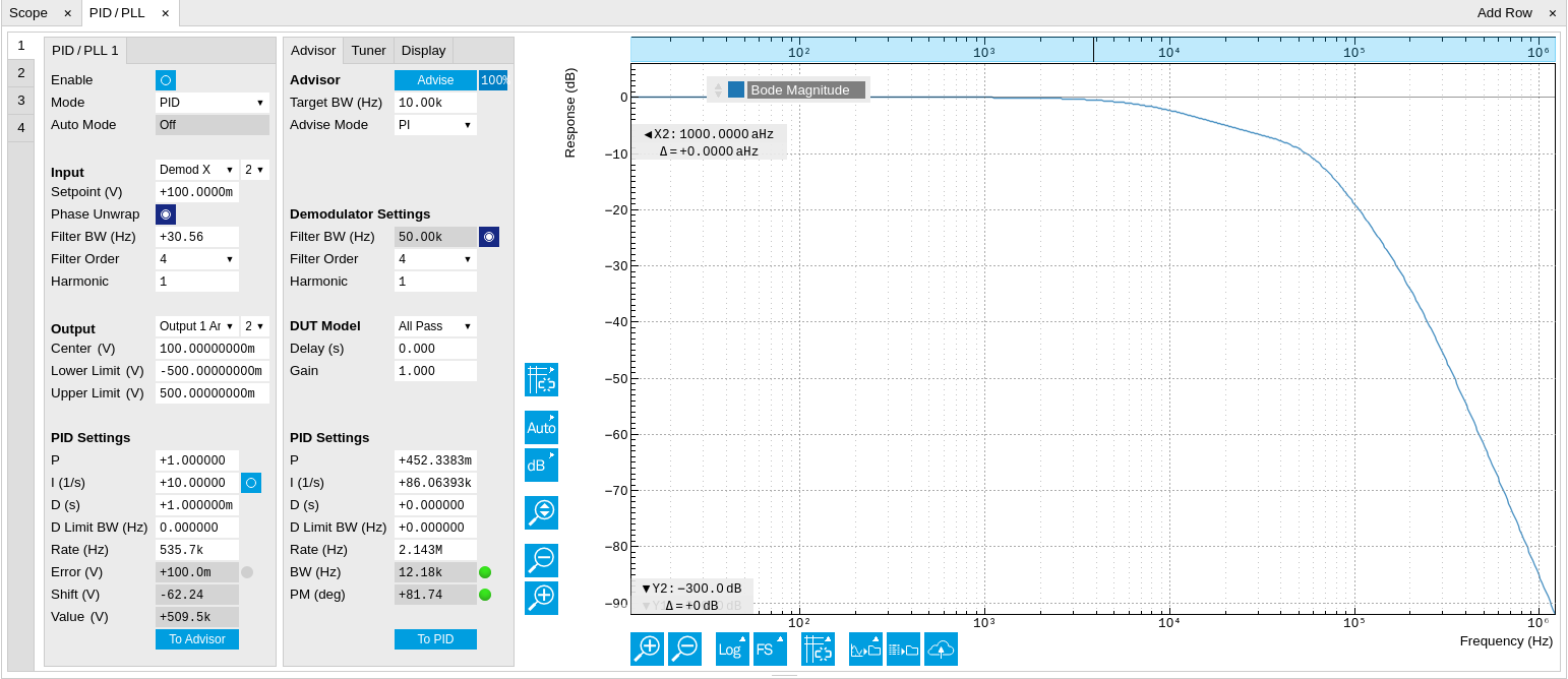
a numerical optimization algorithm. Figure 4 shows a typical view of the PLL tab
after the Advisor has finished. The Advisor tries to match or exceed the
target bandwidth in its simulation. The achieved bandwidth can be read
from the BW (Hz) field, or directly from the 3 dB point of the simulated
Bode plot on the right. The Phase Margin value of the simulation is
displayed in the PM (deg) field and should exceed 45° to ensure stable
feedback operation without oscillations. Once you are satisfied with the
Advisor results, click on the
button to have the Advisor find a set of feedback gain parameters using
a numerical optimization algorithm. Figure 4 shows a typical view of the PLL tab
after the Advisor has finished. The Advisor tries to match or exceed the
target bandwidth in its simulation. The achieved bandwidth can be read
from the BW (Hz) field, or directly from the 3 dB point of the simulated
Bode plot on the right. The Phase Margin value of the simulation is
displayed in the PM (deg) field and should exceed 45° to ensure stable
feedback operation without oscillations. Once you are satisfied with the
Advisor results, click on the  button to transfer the feedback gain parameters to the physical PLL
controller. To start PLL operation, click on the Enable button at the
top of the PLL tab.
button to transfer the feedback gain parameters to the physical PLL
controller. To start PLL operation, click on the Enable button at the
top of the PLL tab.
| Tab | Sub-tab | Section | # | Label | Setting / Value / State |
|---|---|---|---|---|---|
| PLL | Advisor | Advisor | 1 | Target BW (Hz) | 1 k |
| PLL | Advisor | DUT Model | 1 | DUT Model | Resonator Frequency |
| PLL | Advisor | DUT Model | 1 | Res Frequency (Hz) | 1.8 M |
| PLL | Advisor | DUT Model | 1 | Q | 12.8 k |
| PLL | Advisor | Advisor | 1 | Advise | click |
When the PLL is locked, the green indicator next to the label Error/PLL Lock will be switched on. The actual frequency shift is shown in the field Freq Shift (Hz).
Note
At this point, it is recommended to adjust the signal input range by
clicking the Auto Range  button in the Lock-in tab. This often increases the signal-to-noise
ratio which helps the PLL to lock to an input signal.
button in the Lock-in tab. This often increases the signal-to-noise
ratio which helps the PLL to lock to an input signal.
The easiest way to visualize the frequency drift is to use the Plotter
tool. The frequency can be added to the display by using the Tree
Selector
to navigate to Demodulator 1 → Sample and selecting Frequency. The
frequency noise increases with the PLL bandwidth, so for optimum noise
performance the bandwidth should not be higher than what is required by
the experiment. The frequency noise also scales inversely with the drive
amplitude of the resonator.