Boxcar Averager
Note
This tutorial is applicable to MFLI Instruments with the MF-BOX Boxcar Averager option installed.
Goals and Requirements
This tutorial explains how to set up the MF-BOX boxcar averager for measuring periodic signals with low duty cycles. The advantages of using the boxcar averager over a digital scope or a lock-in amplification technique will be explained and demonstrated.
The relationship between duty cycle and signal energy at the fundamental frequency is almost linear. For instance, a rectangular pulse signal with a 50% duty cycle will only retain about one-third of its amplitude at the fundamental frequency. If the duty cycle is halved, the signal at the fundamental frequency is also reduced by half. Consequently, lock-in amplification, which relies on measuring the signal's amplitude at the fundamental frequency, may not always be the most effective method for recovering signals when the waveform has a duty cycle of less than 50%. In such instances, boxcar averaging can offer a more efficient measurement approach. When a signal's power is distributed across various harmonic components in the frequency spectrum without any dominant peak, employing a boxcar detection scheme could be a wiser choice to achieve the optimal signal-to-noise ratio (SNR).
To perform the measurements in this tutorial, a 3rd-party programmable arbitrary waveform (AWG) generator for narrow pulse generation is required.
Preparation
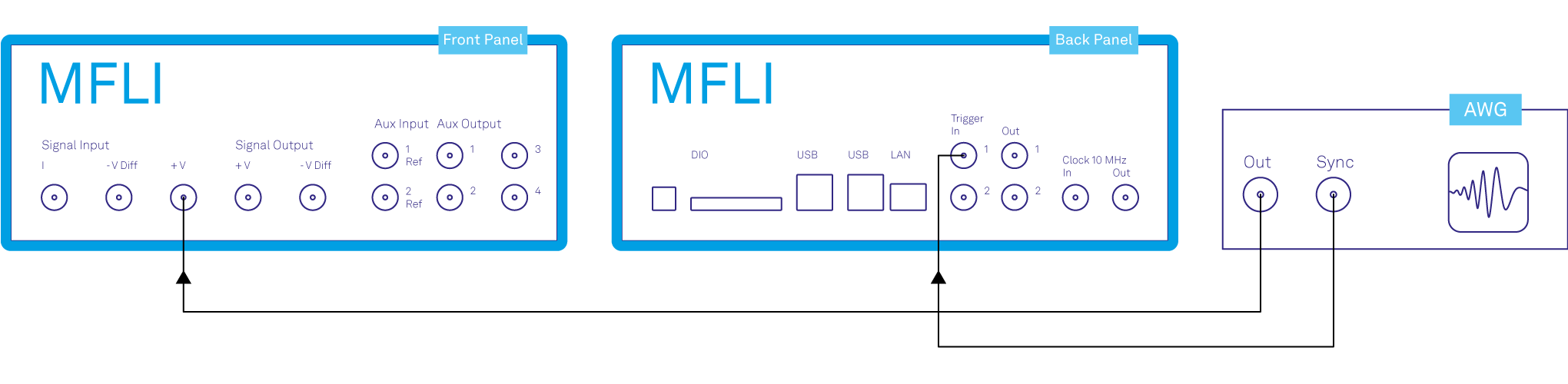
Set up the connection from the AWG to the MFLI as shown in Figure 1. Ensure that the MFLI unit is powered on and connected via USB to your host computer or via Ethernet to your local area network (LAN) where the host computer resides. After starting LabOne, the default web browser opens with the LabOne graphical user interface.
The tutorial can be started with the default instrument configuration (e.g. after a power cycle) and the default user interface settings (e.g. as is after pressing F5 in the browser).
Low Duty Cycle Signal Measurement
There are several ways to measure a low duty cycle signal using the MFLI instrument. One straightforward approach is to utilize the Scope tool within the LabOne interface, to visualize the sampled signal in the time domain. However, when dealing with signals where the amplitude is small or noise backgrounds are large, accurately measuring these signals can be challenging. In such cases, boxcar averaging becomes particularly beneficial, offering improved measurement capabilities.
Narrow Pulse Signal Generation
The initial step involves generating a test signal. Using the external arbitrary waveform generator, we generate a gaussian pulse train with the following specifications.
| Pulse Specification | Section |
|---|---|
| Pulse Type | Gaussian |
| Amplitude | 7 mVpeak |
| Frequency | 10 kHz |
| Duty Cycle | < 5% |
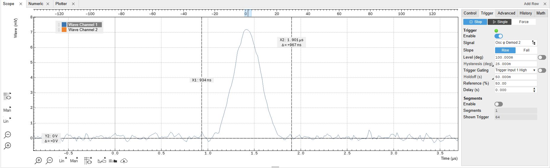
The LabOne Scope on the MFLI can be used to observe the generated pulsed waveform. Connect the output of the AWG directly to Voltage Input of the MFLI instrument. The Scope settings in LabOne are given in the table below and shown in Figure 2. Additionally, the AWG provides a TTL synchronization signal to be connected to one of the Trigger Inputs (back panel). This trigger signal is used as an external reference to lock to the repetition rate of the pulse train.
To analyze the pulse waveform using the boxcar averager, the MFLI instrument first has to lock to the trigger signal of the pulse train (i.e. its repetition rate). This is done using the Ext Ref mode. The trigger signal is fed to the Trigger 1 or 2 connector on the back panel which can be an analog signal or a TTL signal. The workflow to set up an external reference is shown in External Reference tutorial. In this tutorial, we use the 2nd demodulator to lock to the external reference, which in turn uses the 1st oscillator to map the external frequency.
| Tab | Sub-tab | Section | # | Label | Setting / Value / State |
|---|---|---|---|---|---|
| Lock-in | All | Voltage Input | 1 | AC | ON |
| Lock-in | All | Voltage Input | 1 | 50 Ω | OFF |
| Lock-in | All | Voltage Input | 1 | Range | 10 mV |
| Scope | Control | Vertical | Channel 1 | Voltage Input 1/ON | |
| Scope | Trig | Trigger | Signal | Osc φ Demod 2 | |
| Scope | Trig | Trigger | Enable | ON | |
| Scope | Run/Stop | ON |
On the Scope plotting area, one should now be able to observe a waveform similar to the one in Figure 2. The Scope is set to self trigger at every cycle of the oscillator phase. Use the horizontal zoom to focus on a single period. This can be done by rolling the mouse wheel forward to zoom in the horizontal axis. To zoom in on the vertical axis, press down the Shift key and roll the mouse wheel. One can also recenter the waveform by pressing on the left mouse button and dragging the Scope plot area. In cases where the noise doesn't allow to resolve the pulses properly, the averaging function of the Scope can be used to improve the sharpness.
Note
Pulsed or low-duty cycle signals often contain high frequency components that can exceed the fundamental frequency. When using the MF-BOX Boxcar Averager, it's important to ensure that incoming signals fall within the Nyquist limit of the instrument, which is approximately 30 MHz due to its 60 MSa/s input sampling. This consideration helps maintain the integrity of the measurement by preventing potential aliasing or other artifacts.
![]()
Boxcar Integration
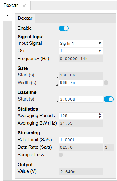
Figure 3 shows the LabOne Boxcar tab. Either the Current Input or the Voltage Input can be selected as the input signal; the boxcar averager integrates and normalizes a section of the input signal and generates an output signal in units of volt (V) or ampere (A). In this example, we will use the Voltage Input. The amplitude value of each sample within the integration window is summed and output from the Adder after each period. This sum is then normalized by the Boxcar window's width. The integration window must be set manually in the Start (deg or s) and Width (deg or s) fields. Additionally, a reference oscillator must be chosen; here, we utilize the oscillator 1 locked to the external reference. The position and width of the integration window can be manually set. To determine the desired values, two possible workflows can be employed: using the Scope or the Sweeper. To further increase the SNR, a moving average filter can be applied to the boxcar output. To do so, one can increase the number of averaging periods. The number of averaging periods indicates how many subsequent periods the integrated values are averaged before outputting the final result. If the averaging periods are set to 1, each consecutive integrated value is output. Increasing the number averaged periods has the effect of improving the SNR at the cost of measurement time, since a longer time is necessary before the result is calculated - similar to the compromise between measurement speed and noise rejection when setting a certain low-pass filter bandwidth in a lock-in measurement. A certain number of averaging period results in an equivalent averaging bandwidth determined by the repetition rate and the number-of-averaging periods (for additional details please refer to the Principle of Boxcar Averaging white paper). To ensure proper streaming of the measurement results to the computer, a large enough Rate Limit must be set (typically two times larger than the averaging bandwidth)
Configuring the Boxcar Integration Window With the Scope
The configuration of the Boxcar averager with the Scope can be very convenient, especially in cases where the amplitude of the pulse train is well above the noise floor. For the configuration of the Start and Width with the Scope, we set the units to seconds (s) in the boxcar tab. We then record a Scope shot with the Scope tab, making sure that the scope is set to Trigger to the correct Oscillator phase, in our case Osc φ Demod 2. By zooming in around the pulse closest to the time 0 of the Scope time axis in the positive times region, we can then move the vertical cursors and set them around the pulse, copying the displayed values to the Start (first cursor) and Width (Δ) settings in the Boxcar Tab. This setup is shown in Figure 2, with the corresponding boxcar settings in Figure 3. By enabling the Boxcar, the data is now streamed to the computer.
Configuring the Boxcar Integration Window With the Sweeper
Alternatively to the Scope, The boxcar averager can be effectively configured using either the Scope or the Sweeper tool. The Sweeper approach is particularly advantageous when the SNR of the pulse train is too low for clear visualization on the Scope, as it allows for improved SNR by sweeping the Start position of the boxcar gate, offering a better pulse profile than a single Scope snapshot would. Importantly, the Sweeper scans the boxcar window's Start position as a function of the phase of the reference oscillators, and the results are displayed in degrees, which provides a phase-based view of the signal characteristics.
To begin, ensure the Boxcar function is disabled, as this is crucial for adjusting certain parameters. Next, navigate to the Boxcar tab and set the Start and Width units to degrees (deg). This mapping uses the phase of the reference oscillator, where a full period corresponds to 360 degrees, allowing you to set the integration window relative to the reference signal’s phase.
Note
The Boxcar must be disabled to edit both the Start and Width value in different units.
Once units are set, adjust the Width of the boxcar gate to the smallest possible value by entering 0, which automatically sets the window size to maximize resolution. Also, set the number of averaging periods to your desired value for proper signal averaging. After these initial configurations, enable the Boxcar function to activate the averaging process and adjust the rate limit according to your measurement requirements for optimal performance.
With these preparations complete, open a Sweeper instance and choose the boxcar window Start as the swept parameter. As a first step, conduct a coarse sweep across the full 360-degree range to identify the general phase delay where the pulse occurs, as shown in Figure 4.
![]()
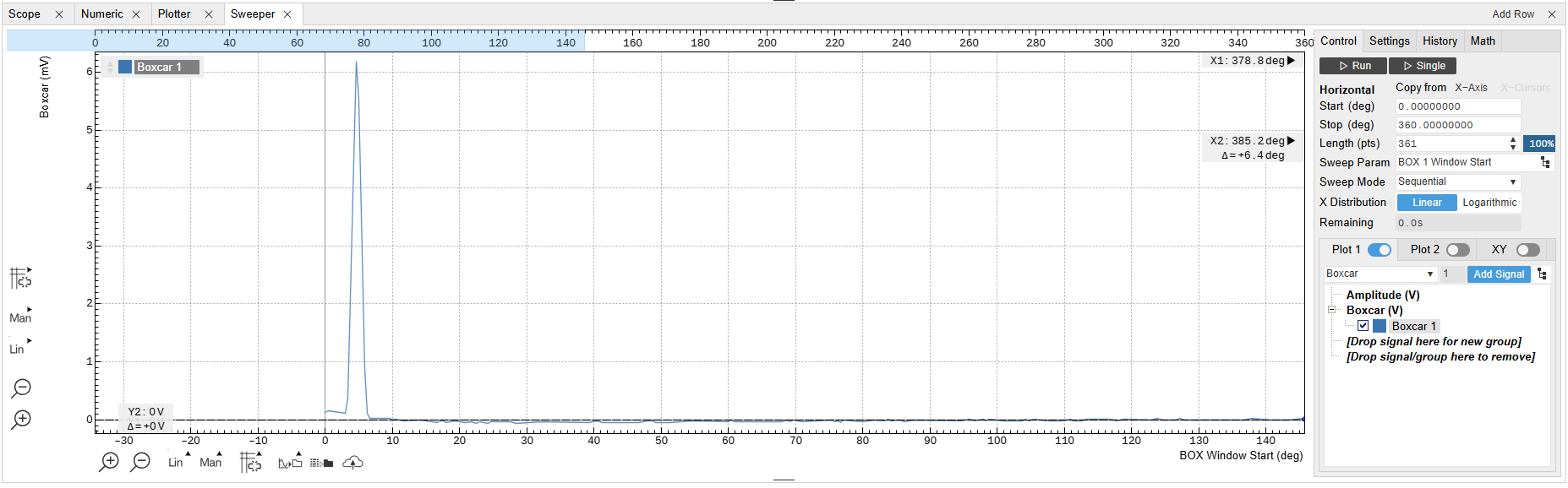
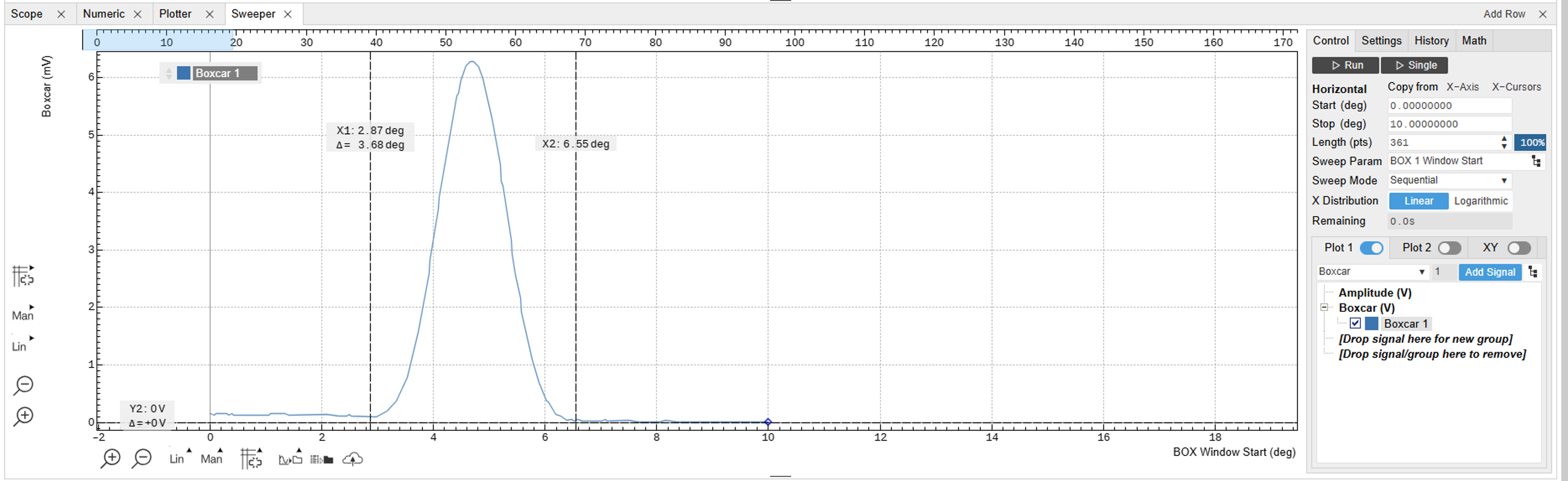
Upon identifying the pulse region, perform a narrower, more detailed sweep around the phase region where the pulse appears Figure 5. Once you have the refined sweep results, copy the displayed Start (first cursor) and Width (Δ) values to the corresponding fields in the Boxcar tab to complete the configuration.
![]()
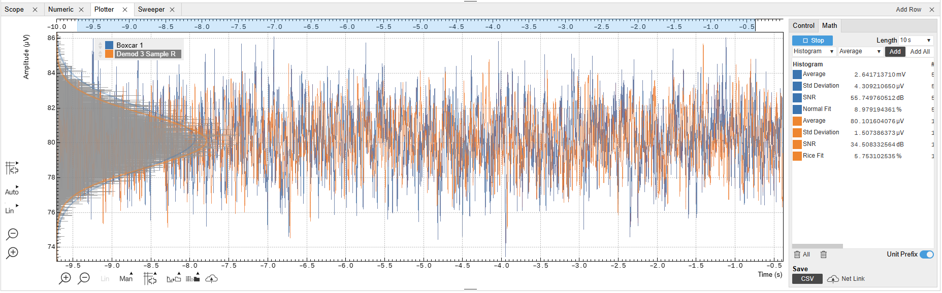
The result of the integration can also be shown graphically using the Plotter tool as shown in Figure 6. As a comparison, the lock-in demodulation of the same pulse train - where the lock-in low pass filter bandwidth is set equal to the boxcar averaging bandwidth for a fair comparison - is overlaid. Thanks to the fitting tool, the SNR of the two measurement approaches can be directly compared. As clearly visible, for a signal with these characteristics, boxcar averaging turns out to be the better measurement approach.
![]()
Baseline Suppression
Baseline subtraction is an additional feature of MF-BOX the boxcar averager that enhances the accuracy of signal measurements by removing unwanted background noise or drift. In this process, the boxcar averager identifies a section of the signal considered as the baseline, often representative of the noise level or underlying trends unrelated to the primary signal of interest. This baseline is then subtracted from the entire signal, effectively isolating the desired signal components.
This feature is particularly beneficial for pulse-to-pulse relative measurements, wherein the gate is set on one pulse and the baseline on another, providing an output that directly reflects the difference between the two. An example application where baseline subtraction on consecutive pulses is particularly useful is in pump-probe spectroscopy, where distinguishing subtle differences between consecutive pulses is desirable.
To set phase or delay of the baseline integration window, simply enter the desired value in the corresponding field and toggle the switch to enable or disable the subtraction. The Width of the baseline window is equal to the gate window by default.