Simple Loop¶

Preparation¶

In this tutorial you generate a signal with the HF2 Instrument and measure that generated signal with the same Instrument. This is done by connecting Signal Output 1/Out with Signal Input 1/+In with a BNC cable. This tutorial shows a single-ended operation, meaning that there is no signal going into the Signal Input 1/-In connector. For proper operation, the Channel 1 must be set to single-ended operation, or alternatively the Input 1 - connector must be shorted to ground using a male shorting cap. Optionally it is possible to connect the generated signal at Output 1 to an oscilloscope by using a T-piece and an additional BNC cable.

Figure 1: Tutorial

Note

This tutorial is both for HF2LI Lock-in Amplifier and HF2IS Impedance Spectroscope users.

Connect the cables as described above. Make sure the HF2 unit is powered on, and then connect the HF2 to your computer with a USB 2.0 cable. Finally launch LabOne (Start Menu/Programs/Zurich Instruments/LabOne User Interface HF2).

Generate the Test Signal¶

Apply the following settings in order to generate a 2.5 MHz signal of 0.5 V amplitude on Signal Output 1/Out.

Open the Lock-in tab and set frequency of Oscillator 1 to 2.5 MHz: click on the field, enter "2.5 M" or "2.5E6" and press <TAB> on your keyboard to confirm the data
In the Output 1 section, set the Range drop-down of 1 V
Without HF2-MF option: In the Output 1 section, set the amplitude to 0.5 V by entering 0.5 followed by a <TAB>
With HF2-MF option: In the Output Amplitudes section, set Amp 1 (Vpk) of demodulator 7 to 0.5 V by entering 0.5 followed by a <TAB>.
By default all physical outputs of the HF2 are inactive to prevent damage to connected circuits. Now turn on the main output switch by clicking on the button labeled "On".
If you have an oscilloscope connected to the setup, you are able to see your generated signal

Table 1: Settings: generate the test signal

Output 1 range	1 V
Oscillator 1 Frequency	2.5 MHz
Demodulator 7 Amp 1	0.5 V
Output 1	ON

Acquire the Test Signal¶

Next, you adjust the input parameters in order to acquire signals with the appropriate input range. To do this, you switch the signal source and the trigger of the Scope to Signal Input 1. Then you adjust the Signal Input 1 range to 1 V.

Table 2: Settings: acquire the test signal

Scope Signal Input	Signal Input 1
Scope Trigger Signal	Signal Input 1
Scope Sampling Rate	210 MS, 10 us
Run / Stop	RUN
Signal Input 1 range	1 V
Signal Input 1 AC / 50 / Diff	ON / OFF / OFF

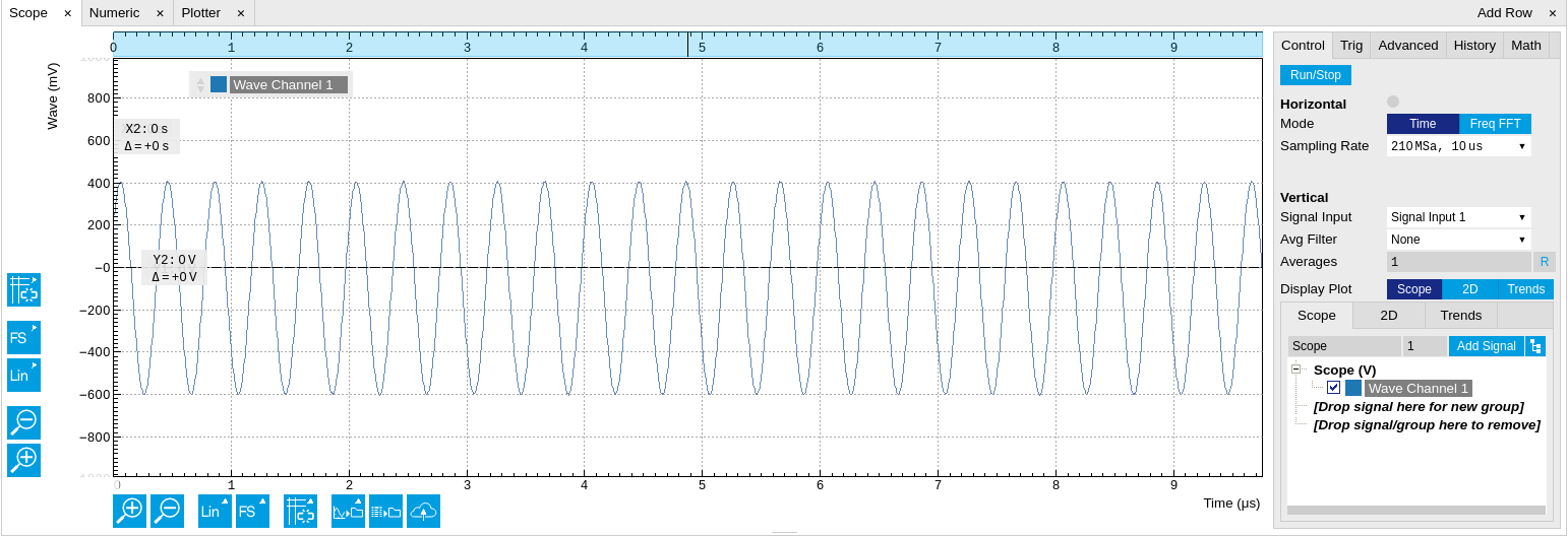
Figure 2: LabOne UI displaying the acquired signal

The Scope displays the measured signal at Input 1. Having set the input range to 1 V ensures that no signal clipping occurs. If you try and set the input range to 0.3 V you see the effect in the Scope window. Note how the red "Over" LEDs on the front panel of the HF2 indicates the error condition and the set OV (OVI) status flag on the right-bottom corner of the window. Set back the input range to 1 V and then clear the flag by clicking . The Scope is a very handy tool to quickly check settings before proceeding to more advanced measurements, please refer to Scope Tab for a full description of features available in the Scope.

Measure the Test Signal¶

Next you use the demodulators of the HF2 to measure acquired test signal. You will use the Numeric and the Plotter tab from the LabOne user interface. First apply the following settings (choose any of the demodulators 1 to 6).

Table 3: Settings: measure the test signal

Filter BW 3 dB	7 Hz (approximated to 6.8 Hz)
Filter order	2
Data transfer rate	100 Hz (approximated to 112 Hz)
Data transfer enable (En)	ON

These settings set the demodulation filter to second-order low-pass operation with a 7 Hz bandwidth. The corresponding time constant can be obtained easily by clicking on the label on top of the bandwidth setting column according to Equation 3 provided in Signal Processing Basics. The output of the demodulator filter is read out with 100 Hz, implying that 100 data samples are sent to the host PC per second. These samples are viewed in the Numeric and Plotter tab that we examine next.

The Numeric tool provides the space for 6 measurement panels corresponding to the 6 demodulators. Each of the panels has the option to display the samples in Cartesian (X,Y) or polar format (R,THETA). The unit of the (X,Y,R) values is V_RMS.

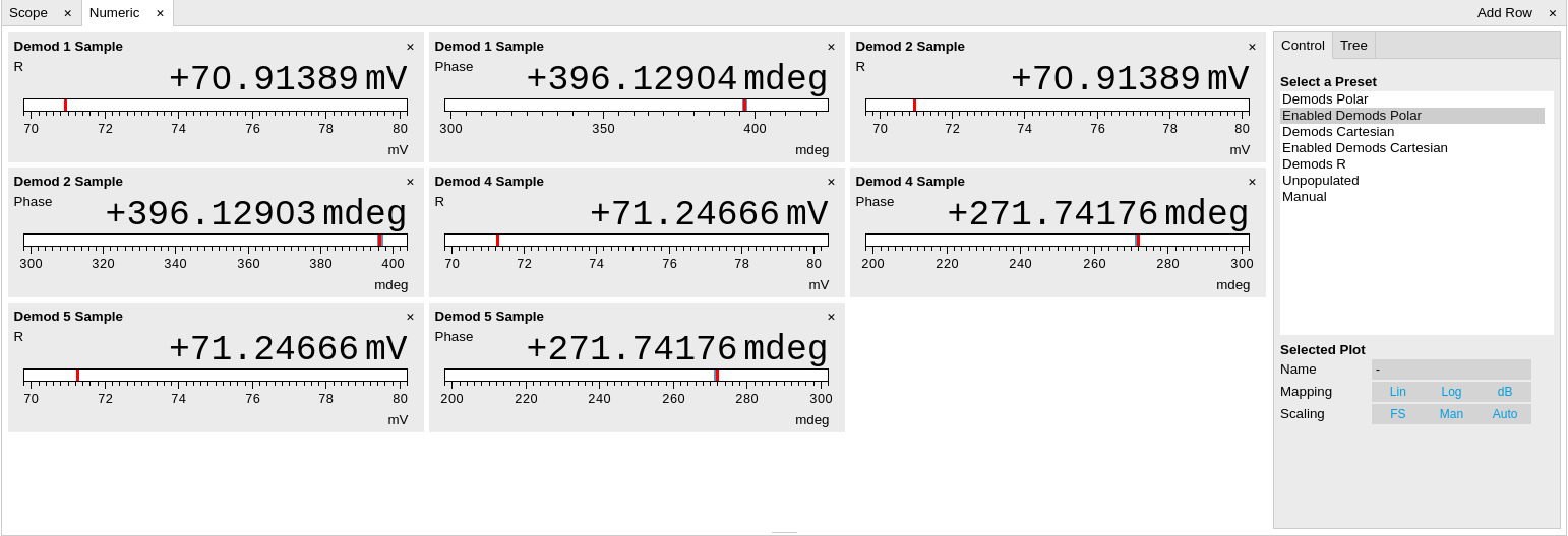
If you wish to play around with the settings, you could now change the amplitude of the generated signal, and observe the effect on the demodulator output.

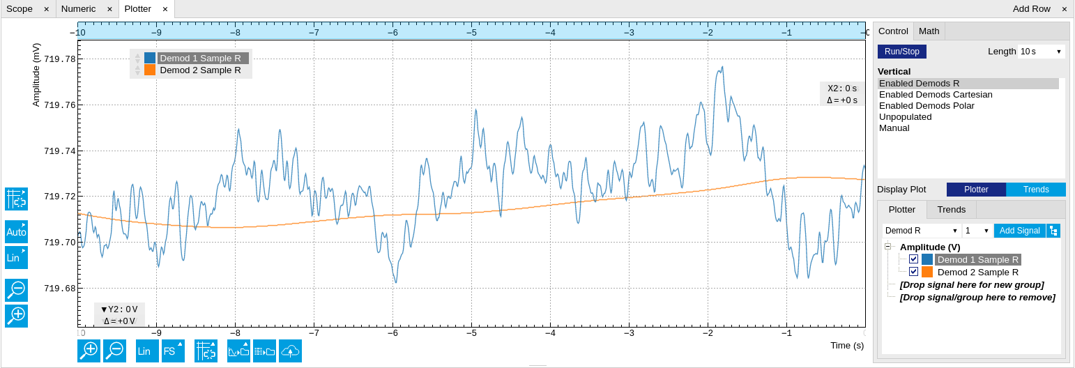
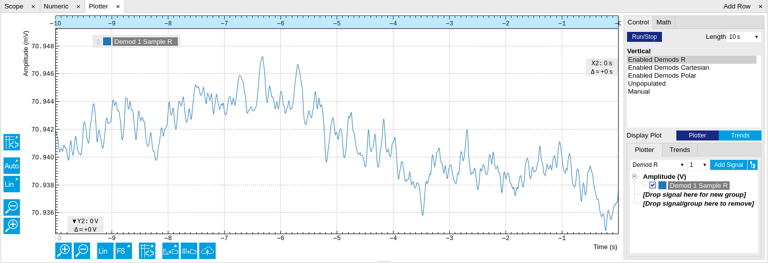
Next, we’ll have a look at the tab. This tab provides a time plot of the demodulator outputs. It is possible to plot up to 6 signals continuously as (X,Y) or (R,THETA) pairs, to set different scales, or to make detailed measurements with 2 cursors. For a detailed description of the functionality available in the Plotter please see Plotter Tab and Plot Functionality.

Figure 4: LabOne Plotter view with plot of demodulator 1 output (TC = 10 ms)

Different Filter Settings¶

As last step of this tutorial you change the filter settings and see the effect on the measurement results. For instance you change the time constant of the integration to 2 seconds.

Table 4: Settings: changing the filter settings

Time constant (TC)	2 s
Filter slope	12 dB/Oct
Resulting measurement bandwidth (BW)	\~51 mHz

Increasing the time constant increases the integration time of the demodulators smoothing out the demodulator outputs. This averages the noise over time and the output of the filters is more stable. This manifests itself in a smoother curve of the demodulator data but also in a larger number of stable digits in the Numeric tab.