HF2LI First Time User
This tutorial covers basic operation of the HF2LI lock-in amplifier with the LabOne User Interface.
The LabOne User Interface is provided as the primary interface to the HF2LI but it is not the only program that can run the instrument. Typically, the user will use LabOne UI to set up the instrument and then either use LabOne UI to take the measurements or run (possibly concurrently) some custom programs.
Note
This tutorial aims to give a walk-through of the main features of the LabOne User Interface. Please also see User Interface Overview for an overview of the UI’s layout and Functional Description LabOne User Interface in general for a thorough description of all the available settings available in LabOne UI for your instrument.
The Lock-in Tab
Open the Lock-in tab by clicking on the Lock-in icon on the left side of the user interface. If you find the Lock-in MF tab, it means that the instrument has the HF2-MF option installed. Lock-in Tab provides the full documentation of the Lock-in tab while Lock-in Tab (HF2-MF option) describes the Lock-in MF tab.
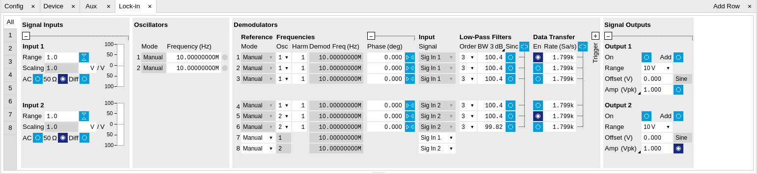
The Signal Inputs section contains a Range that can be set to a value between 1 mV and 1.6 V, the largest amplification of the input signal is achieved for 1 mV. The input has protection diodes that clip signals with amplitude above 5 V.
Warning
Please respect the compliance to the maximum ratings Maximum ratings to prevent damage to the instrument.
The AC button sets the coupling type: AC coupling has a cutoff frequency of 1 kHz. The AC coupling consists of a blocking capacitor between two input amplifier stages: this means that a DC signal larger than 5 V will saturate the front amplifier even if AC coupling is enabled. The Diff Differential mode button sets single-ended/differential measurement mode: in the differential mode, the voltage difference between the +In and -In is amplified whereas in single-ended mode, the voltage at the +In connector is amplified. The 50 Ω button toggles the input impedance
between low (50 Ω) and high (approx 1 MΩ) input impedance. 50 Ω input impedance should be selected for signal frequencies above 10 MHz to avoid artifacts generated by multiple signal reflections within the cable. With 50 Ω input impedance, one will expect a reduction of a factor of 2 in the measured signal if the signal source also has an output impedance of 50 Ω.
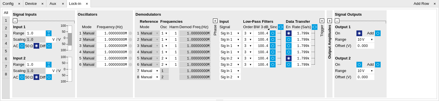
Next, one finds the Oscillators section used to control the frequency for the demodulation with an internal reference. For the purpose of this tutorial, set the frequency of oscillator 1 to 1 MHz.
Under the section Demodulators the user can select which harmonics and filter bandwidths to use for demodulation. It is not uncommon to need to measure different harmonics (integer multiples of the fundamental frequency, in this case 1 MHz). Select the harmonic (Harm) to 1 for the first demodulator (the first line), set the filter order to 4 (this corresponds to a filter steepness of 24 dB/oct or 80 dB/dec, an attenuation of 104 for a tenfold frequency increase) and type 10 Hz into the BW control (the digital filters of the HF2 are described in Discrete-Time Filters). Users are sometimes interested in the second harmonic that may be generated by nonlinear processes in their device under test: select harmonic 2 for the second demodulator and type the same values for the filter order and BW as in the previous case. You can also measure the same fundamental harmonic with a larger bandwidth: set harmonic to 1, order to 24 dB/oct and BW to 1 kHz for the third demodulator. Measuring with different bandwidths can provide the signal average and transient values. Click on the enable button next to the filters to read out the values from the 3 demodulators.
Next, set the Trigger to Continuous and the Rate to 7.20 kSa/s (rate settings can only be sub-multiples of 460 kSa/s, the maximum readout rate for one demodulator): in this case, the HF2LI will send the demodulated signal sampled at this rate through the USB. Due to the finite bandwidth of the USB connection the maximum cumulative demodulator sample rate is 700 kSa/s, which can be split over the active demodulators, see Maximum sample readout rate. In this example we’re using 3 active demodulators, therefore, since the sample rates are sub-multiples of 460 kSa/s the maximum possible readout rate for each demodulator is 230 kSa/s. Note that, according to the Nyquist sampling theorem , the sampling rate should be at least twice as fast as the maximum frequency present in the signal, in order to reconstruct the demodulated signal (this is not important if you only need one data point or the standard deviation of the demodulated signal). Since the low-pass filters do not have an infinite roll-off (the attenuation is not infinite past the filter’s 3 dB frequency), it is common to set the sampling rate to about 8 times higher than the filter bandwidth.
Next, we configure the HF2 to output a 1 MHz signal on its Signal Output 1/Out connector. In case you have the HF2-MF Option installed, go to the Signal Outputs section, set the excitation amplitude Amp (Vpk) to 100 mV and the output range to be the smallest possible but at least twice as large as than the amplitude for minimum harmonic distortion. Connect Signal Output 1 to Signal Input 1 +In with a BNC cable and click on the On button in the LabOne Signal Outputs section of Output 1. With the HF2-MF Option installed, first go the Output Amplitudes section, set the signal amplitude Amp 1 (Vpk) of demodulator 7 to 100 mV and enable the button next to the amplitude field. Connect Signal Output 1 to Signal Input 1 +In with a BNC cable and click on the On button in the LabOne Signal Outputs section of Output 1.
The Numeric Tab
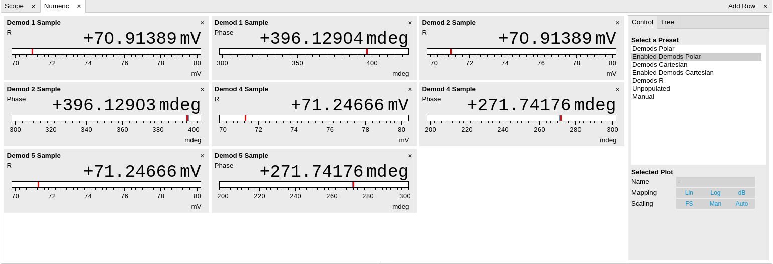
In the Numeric tab, you should read 71 mV RMS for the R component of demodulator 1, (demodulating at 1 MHz). The RMS corresponds to the 100 mV divided by √2. The phase value will depend on the BNC cable length (for lengths shorter than one meter, the phase is approximately a few degrees). Demodulator 3 (also at 1 MHz) will show the same amplitude, but the digits fluctuate more, since the measurement bandwidth and therefore the noise, is larger. Demodulator 2 reads only a few MUV because at 2 MHz (the second harmonic) there is only a little component of the signal, coming from the harmonic distortion of the HF2LI output and input stages.
The Plotter Tab
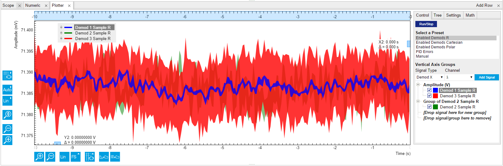
Now open the Plotter tab. Here one can display the demodulated values over time. Select Enabled Demods R from the Presets and click on Run/Stop to start the acquisition. The demodulated traces for these three demodulators are displayed, offset to one another: as before, demodulators 1 and 3 have the same average value, but a larger noise amplitude is clearly visible in the third trace. In Plot Functionality you can find a detailed description of the functions of the plot window. For instance you can find there ways to change the horizontal and vertical scales, to remove offsets in the plot, and to use the cursors for exact measurements. The amount of stored data depends on the set Window Length in the Settings sub-tab.
The Scope Tab
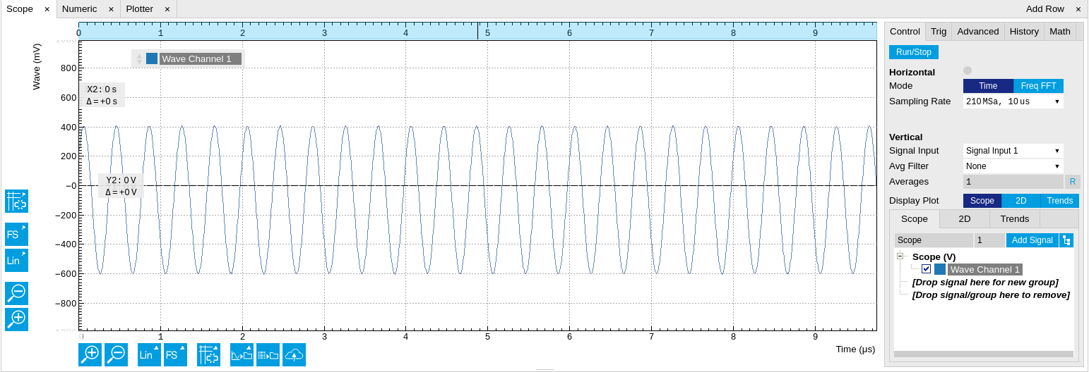
Let us proceed to the Scope tab. The Scope can be used to display the signal at the signal inputs and outputs of the HF2LI. It has a 2048 point wave memory that is useful for visualizing the raw signal. It also replaces the need for an external oscilloscope. Select Signal Input 1 in the Vertical section of the Control sub-tab, Signal Output 1 as the Signal in the Trigger sub-tab and press the Run/Stop button. The 1 MHz input signal is visible as 10 full cycles if the Sampling Rate is set to 210 MS, 10 μs in the Control sub-tab. Decreasing the sampling rate to display a longer time interval should be done carefully because it may lead to aliasing: for instance setting the sampling rate to 26 kSa/s, 80 ms, will produce a correctly looking sinusoidal, but at the wrong frequency. The BW Limit button in the Advanced sub-tab may reduce aliasing effects without removing them completely.
The update rate of the oscilloscope frames is controlled by the Holdoff time in the Trigger sub-tab: the minimum interval between two traces is 10 ms. This is a low value which increases the load of the USB bandwidth and may lead to USB sample loss - therefore avoid using small hold off values if not needed.
You can go from the time domain display to a frequency domain display by selecting the Freq Domain FFT Mode in the Control sub-tab. The frequency resolution is coarse because the time trace contains 2048 points. Averaging of the Fourier power spectra can be enabled to increase the SNR ratio.
The Sweeper Tool

Next is the Sweeper tool: it turns the HF2LI into a frequency response analyzer, giving the transfer function of a device under test in the form of a Bode plot. In AFM applications this is useful to easily identify the resonance frequency of a cantilever as well as the phase delay. The sweeper tool can also be used to sweep parameters other than frequency: phase, time constant, amplitude and auxiliary output voltage.
As a frequency sweeper example, we will execute a logarithmic sweep of 100 points between 1 kHz and 1 MHz. In the Horizontal section, set the sweep range Start to 1 kHz and Stop to 1 MHz, 100 points and enable the Log Sweep. Click on Run/Stop for continuous sweeping or on Single for a single sweep. Toggle the AC input coupling in the Lock-in settings, and observe the attenuation in the response at 1 kHz in AC coupling, since the AC coupling has a cutoff frequency of approximately 1 kHz. In the History sub-tab, the measurement that is displayed can be saved to a data file in ASCII format. There it is also possible to declare one out of several measured traces as a reference by selecting the trace in the list and clicking on Reference. The selected trace then appears below the list, and next to it there is the enable button for the reference mode. In reference mode, all traces in the plot are divided by the reference trace.
During the logarithmic sweep the NEPBW (noise equivalent power bandwidth) is adjusted for each frequency point and displayed under the Filters BW field under the Lock-in tab. The adjustment is due to the fact that the sweep is logarithmic and the sweep frequency steps are not equally spaced. In order to account for all signal power (and power densities), the measurement bandwidth must be changed accordingly. This can be done automatically by going from Application Mode to Advanced mode in the Settings sub-tab, and there selecting Auto as the Bandwidth Mode. For an explanation of the NEPBW, see Signal Bandwidth chapter. Note that in this configuration, if the signal to noise ratio is large, there will not be any effect when disabling Auto BW, since the noise signal is negligible when measured with (almost) any NEP bandwidth. Averaging can also help to improve the signal-to-noise ratio during the sweep.
As an example of noise measurement, disconnect the BNC cable from Signal Output 1 and connect it to Signal Output 2. In the Lock-in tab, turn off the Signal Output 1, and generate a 100 kHz / 100 mV excitation Signal Output 2 (remember to turn on the output in the Signal Outputs section). In the frequency sweeper perform a single sweep with Auto BW enabled. A relatively wide peak will appear at 100 kHz, as the measurement was performed with wide NEPBW. Switch the X scaling to Manual and zoom into the region around 100 kHz; click the Copy From Range button to use the new boundaries for the sweep as selected in the graph and again perform a single sweep. The peak at 100 kHz will appear narrow, reflecting the change in the measurement bandwidth.
The Spectrum Tab
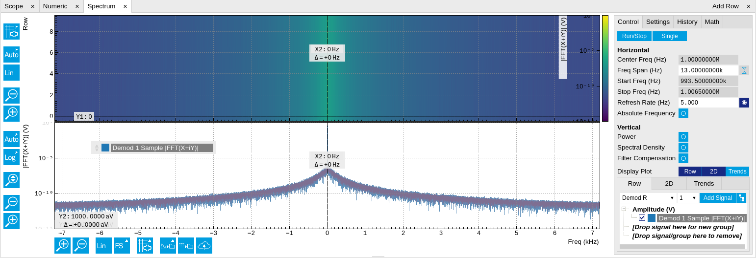
The Spectrum tool (more information (see Zoom FFT)) allows the user to measure the frequency spectrum around a specific frequency: this is done by performing the Fourier transform of the demodulated X and Y (or in-phase and quadrature) components of the signal (more precisely of the quantity X+jY, where j is the imaginary unit). This method is called zoomFFT. The frequency resolution that can be achieved in this way is given by the sampling rate divided by the number of recorded samples, and is therefore much higher than the frequency resolution obtained in the Scope tab. The zoomFFT approach is more efficient than the FFT on raw samples in which one digitizes a long time trace, performs the Fourier transform and retains only the portion of the frequency spectrum of interest while discarding the rest.
We continue from the previous section with the BNC connecting Signal Output 2 to Signal Input 1, and 100 mV, 100 kHz sine wave. In the Lock-in tab, set the oscillator 1 frequency to 101 kHz. Set the Demodulator 1 parameters to filter order 4, filter bandwidth 500 Hz, and Data transfer rate 7.2 kSa/s. In the Spectrum tab, enable Filter Compensation and select Demodulator 1 for Signal Input. A peak appears at 1 kHz to the left of the center frequency. Increasing the number of lines in FFT will result in a finer frequency resolution. The Filter compensation button compensates for the demodulator filter, by dividing the measured spectrum by the demodulator filter transfer function. This is why the input signal does not appear attenuated despite being outside the filter bandwidth (1 kHz and 500 Hz respectively).
The Auxiliary Tab
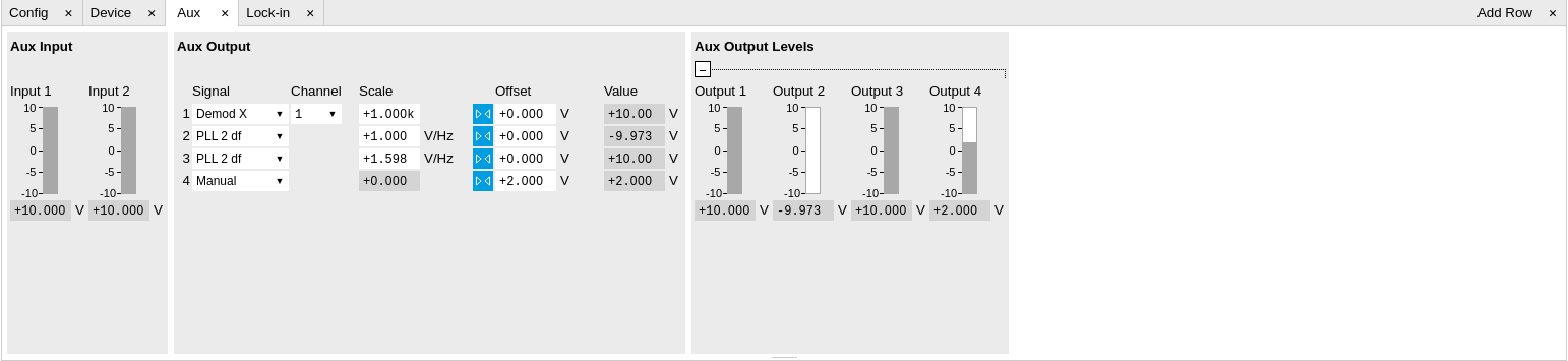
The Auxiliary tab controls the 4 Auxiliary Outputs on the right side of
the HF2LI front panel, as well as the 2 Auxiliary Inputs on the rear
panel. Aux Output 1 is represented by the first line of controls in the
Aux Output section. In order to output the lock-in signal on this
connector, select Demod R from the Signal drop-down menu and set the
channel (i.e., the demodulator number) to 1. Set the Scale factor to 10
V/VRMS: you should read 0.712 V in the output Value (V)
field, which corresponds to the amplitude of the signal as you can read
it in the Numeric tab multiplied by the scale factor. If one is
interested in small variations of the signal amplitude, an offset can be
applied to the output: type –0.712 in Offset (V) or click on the button
 next to the Offset field: Value (V) should now read 0.