Scope Tab

The Scope is a powerful time domain and frequency domain measurement tool as introduced in Unique Set of Analysis Tools and is available on all HF2 Series instruments.

Features

• One input channel with 2 kSa of memory
• 14 bit nominal resolution
• Fast Fourier Transform (FFT): up to 100 MHz span, spectral density and power conversion, choice of window functions
• Sampling rates from 6.4 kSa/s to 210 MSa/s; up to 10 μs acquisition time at 210 MSa/s or 320 ms at 6.4 kSa/s
• 4 signal sources; up to 13 trigger sources and 2 trigger methods `
• Independent hold-off and trigger level settings

Description

The Scope tab serves as the graphical display for time domain data. Whenever the tab is closed or an additional one of the same type is needed, clicking the following icon will open a new instance of the tab.

Table 1: App icon and short description

Control/Tool	Option/Range	Description
Scope		Displays shots of data samples in time and frequency domain (FFT) representation.

Figure 1: LabOne UI: Scope tab - Time domain

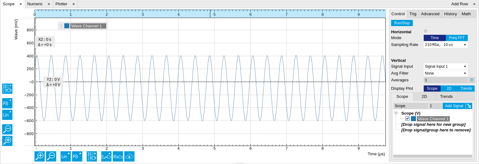
The Scope tab consists of a plot section on the left and a configuration section on the right. The configuration section is further divided into a number of sub-tabs. It gives access to a single-channel oscilloscope that can be used to monitor a choice of signals in the time or frequency domain. Hence the X axis of the plot area is time (for time domain display, Figure 1) or frequency (for frequency domain display, Figure 3). It is possible to display the time trace and the associated FFT simultaneously by opening a second instance of the Scope tab.

The Scope records data from a single channel at up to 210 MSa/s. The channel can be selected among the two Signal Inputs and the two Signal Outputs. The Scope records data sets of up to 2 kSa samples in the standard configuration, which corresponds to an acquisition time of 10 μs at the highest sampling rate.

Figure 2: Illustration of how the Scope output is generated in BW Limitation and decimation mode when the sampling rate is reduced from the default of 210 MSa/s to 52.5 MSa/s

The frequency domain representation is activated in the Control sub-tab by selecting Freq Domain FFT as the Horizontal Mode. It allows the user to observe the spectrum of the acquired shots of samples. All controls and settings are shared between the time domain and frequency domain representations.

The Scope supports averaging over multiple shots. The functionality is implemented by means of an exponential moving average filter with configurable filter depth. Averaging helps to suppress noise components that are uncorrelated with the main signal. It is particularly useful in combination with the Frequency Domain FFT mode where it can help to reveal harmonic signals and disturbances that might otherwise be hidden below the noise floor.

Figure 3: LabOne UI: Scope tab - Frequency domain

The Trigger sub-tab offers all the controls necessary for triggering on different signal sources. When the trigger is enabled, then oscilloscope shots are acquired whenever the trigger conditions are met. Trigger and Hysteresis levels can be indicated graphically in the plot. A disabled trigger is equivalent to continuous oscilloscope shot acquisition.

Functional Elements

Table 2: Scope tab: Control sub-tab

Control/Tool	Option/Range	Description
Run/Stop		Runs the scope/FFT continuously.
Mode	Freq Domain (FFT)	Switches between time and frequency domain display.
	Time Domain
Sampling Rate	6.4 kSa/s to 210 MSa/s	Defines the sampling rate of the scope. The numeric values are rounded for display purposes. The exact values are equal to the base sampling rate divided by 2^n, where n is an integer.
Sampling Rate		Defines the sampling rate of the scope. The numeric values are rounded for display purposes. The exact values are equal to the base sampling rate divided by 2^n, where n is an integer. Warning: Due to the lack of sample averaging feature, reduced sampling rates can cause aliasing and thus artifacts in the signal spectrum. Currently, the Scope tool only supports sample decimation, but in the future it will also offer sample averaging.
Signal Input	Signal Output 2	Selects the source for the scope input.
	Signal Input 1
	Signal Input 2
	Signal Output 1
Average Filter		Enable Exponential Moving Average (EMA) filter that is applied when the average of several scope shots is computed and displayed. Depending on the mode, the source data for averaging is either the Time or the Freq FFT trace.
	Off	Averaging is turned off.
	On	Consecutive scope shots are averaged with an exponential weight.
Averages	integer value	The number of shots required to reach 63% settling. Twice the number of shots yields 86% settling.
Averages	integer value	The number of shots to average on the device before returning the data.
Reset		Resets the averaging filter.

For the Vertical Axis Groups, please see the table "Vertical Axis Groups description" in the section called "Vertical Axis Groups".

Table 3: Scope tab: Trigger sub-tab

Control/Tool	Option/Range	Description
Trigger	grey/green/yellow	When flashing, indicates that new scope shots are being captured and displayed in the plot area. The Trigger must not necessarily be enabled for this indicator to flash. A disabled trigger is equivalent to continuous acquisition. Scope shots with data loss are indicated by yellow. Such an invalid scope shot is not processed.
Signal		Selects the trigger source signal.
	Off	Switches the scope off.
	Continuous	A new waveform is acquired and displayed after the hold off time. The trigger source is ignored.
	Signal Inputs 1/2	A new waveform is acquired and displayed when the respective Signal Input is matching the trigger condition.
	Signal Outputs 1/2	A new waveform is acquired and displayed when the respective Signal Output is matching the trigger condition.
	Oscillators 1-8	A new waveform is acquired and displayed when the respective Oscillator is matching the trigger condition.
	DIO 0/1	A new waveform is acquired and displayed when the respective DIO signal is matching the trigger condition.
Slope	Falling edge trigger	Select the signal edge that should activate the trigger.
	Rising edge trigger
Level (%)	numeric percentage value (negative values permitted)	Defines the trigger level relative to signal full scale.
Holdoff (s)	numeric value	Defines the time before the trigger is rearmed after a recording event.
Plot Type		Select the plot type.
	None	No plot displayed.
	2D	Display defined number of grid rows as one 2D plot.
	Row	Display only the trace of index defined in the Active Row field.
	2D + Row	Display 2D and row plots.
Active Row	integer value	Set the row index to be displayed in the Row plot.
Track Active Row	ON / OFF	If enabled, the active row marker will track with the last recorded row. The active row control field is read-only if enabled.
Palette	Solar	Select the colormap for the current plot.
	Viridis
	Inferno
	Balance
	Turbo
	Grey
Colorscale	ON / OFF	Enable/disable the colorscale bar display in the 2D plot.
Mapping		Mapping of colorscale.
	Lin	Enable linear mapping.
	Log	Enable logarithmic mapping.
	dB	Enable logarithmic mapping in dB.
Scaling	Full Scale/Manual/Auto	Scaling of colorscale.
Clamp To Color	ON / OFF	When enabled, grid values that are outside of defined Min or Max region are painted with Min or Max color equivalents. When disabled, Grid values that are outside of defined Min or Max values are left transparent.
Start	numeric value	Lower limit of colorscale. Only visible for manual scaling.
Stop	numeric value	Upper limit of colorscale. Only visible for manual scaling.

Table 4: Scope tab: Advanced sub-tab

Control/Tool	Option/Range	Description
FFT Window	Cosine squared (ring-down)	Several different FFT windows to choose from. Each window function results in a different trade-off between amplitude accuracy and spectral leakage. Please check the literature to find the window function that best suits your needs.
	Rectangular
	Hann
	Hamming
	Blackman Harris
	Flat Top
	Exponential (ring-down)
	Cosine (ring-down)
Resolution (Hz)	mHz to Hz	Spectral resolution defined by the reciprocal acquisition time (sample rate, number of samples recorded).
Absolute Frequency	ON / OFF	Shifts x-axis labeling to show the absolute frequency in the center as opposed to 0 Hz, when turned off.
Spectral Density	ON / OFF	Calculate and show the spectral density. If power is enabled the power spectral density value is calculated. The spectral density is used to analyze noise.
Power	ON / OFF	Calculate and show the power value. To extract power spectral density (PSD) this button should be enabled together with Spectral Density.
Persistence	ON / OFF	Keeps previous scope shots in the display. The color scheme visualizes the number of occurrences at certain positions in time and amplitude by a multi-color scheme.
BW Limit	ON / OFF	Select between scope sample decimation and averaging. Averaging avoids aliasing but may conceal single-sample peaks.
Rate		Streaming rate of the scope channels. The streaming rate can be adjusted independent from the scope sampling rate. The maximum rate depends on the interface used for transfer. Note: scope streaming requires the DIG option.

Table 5: Scope tab: History sub-tab

Control/Tool	Option/Range	Description
History	History	Each entry in the list corresponds to a single trace in the history. The number of traces displayed in the plot is limited to 20. Use the toggle buttons to hide or show individual traces. Use the color picker to change the color of a trace in the plot. Double click on a list entry to edit its name.
Length	integer value	Maximum number of records in the history. The number of entries displayed in the list is limited to the 100 most recent ones.
Clear All		Remove all records from the history list.
Clear		Remove selected records from the history list.
Load file		Load data from a file into the history. Loading does not change the data type and range displayed in the plot, this has to be adapted manually if data is not shown.
Name		Enter a name which is used as a folder name to save the history into. An additional three digit counter is added to the folder name to identify consecutive saves into the same folder name.
Auto Save		Activate autosaving. When activated, any measurements already in the history are saved. Each subsequent measurement is then also saved. The autosave directory is identified by the text "autosave" in the name, e.g. "sweep_autosave_001". If autosave is active during continuous running of the module, each successive measurement is saved to the same directory. For single shot operation, a new directory is created containing all measurements in the history. Depending on the file format, the measurements are either appended to the same file, or saved in individual files. For HDF5 and ZView formats, measurements are appended to the same file. For MATLAB and SXM formats, each measurement is saved in a separate file.
File Format		Select the file format in which to save the data.
Save		Save the traces in the history to a file accessible in the File Manager tab. The file contains the signals in the Vertical Axis Groups of the Control sub-tab. The data that is saved depends on the selection from the pull-down list. Save All: All traces are saved. Save Sel: The selected traces are saved.

For the Math sub-tab please see the table "Plot math description" in the section called "Cursors and Math".