Dual-phase Demodulation¶

Note

This tutorial is applicable to all UHFQA Instruments.

Goals and Requirements¶

This tutorial explains how to analyze a pulsed signal using the weighted integration units and record the result with the Result Logger in the Quantum Analyzer Result tab.

The measurements in this tutorial can be performed using simple loop back connections.

Preparation¶

Connect the cables as illustrated below. Make sure that the UHF unit is powered on and connected by USB to your host computer or by Ethernet to your local area network (LAN) where the host computer resides. After starting LabOne the default web browser opens with the LabOne graphical user interface.

Figure 1: UHF connections for the Dual-phase Demodulation tutorial

The tutorial can be started with the default instrument configuration (e.g. after a power cycle) and the default user interface settings (e.g. as is after pressing F5 in the browser).

Continuous Wave Signal Generation¶

First, we enable both outputs of the UHF instrument and the digital oscillator. The first (second) output then generates a cosine (sine) waveform at the frequency defined in the oscillator section.

Table 1: Settings: observe the pulse waveform
Tab	Section	#	Label	Setting / Value / State
In / Out	Signal Outputs	1	On	ON
In / Out	Signal Outputs	1	50 Ohm	ON
In / Out	Signal Outputs	1	Amp (Vpk)	0.5
In / Out	Signal Outputs	1	Amp (Vpk)	ON
In / Out	Signal Outputs	2	On	ON
In / Out	Signal Outputs	2	50 Ohm	ON
In / Out	Signal Outputs	2	Amp (Vpk)	0.5
In / Out	Signal Outputs	2	Amp (Vpk)	ON
In / Out	Oscillators	1	Frequency (Hz)	10M

Copy the following code into the Sequence Editor in the AWG tab.

var result_length = getUserReg(0);
var result_averages = getUserReg(1);

repeat (result_averages) {
  repeat (result_length) {
    startQA(QA_INT_0 | QA_INT_1, true);
    wait(512);
  }
}

Upload this program to the AWG by clicking on "Save" or "To Device". The outputs will generate a continuous waveform at the frequency as configured before, and the sequencer will control only the triggering of the readout and monitor unit. See Architecture and Signalling for an overview of the different functional blocks and internal trigger lines.

There are two nested loops in the sequence above: the number of repetitions in the inner loop is determined by User Register 1 and would correspond to the number of points in a pulsed measurement. The outer loop corresponds to the number of identical repetitions to be performed in order to allow averaging and is determined by User Register 2. For spectroscopy measurements, one is usually interested in a single averaged data point while stepping an external parameter, such as a signal generator frequency. This would correspond to a parameter result_length of 1. Here, we choose a result_length 2, for the practical reason that the final data is more clearly displayed in the QA Result tab. Apply the settings in the following table to configure the AWG output as well as the User Registers.

Table 2: Settings: configure the AWG output and User Registers
Tab	Sub-tab	Section	Label	Setting / Value / State
AWG	Control		Rerun	OFF
AWG	Control	User Registers	Register 1	2 (Length)
AWG	Control	User Registers	Register 2	32 (Averages)

To visualize the generated signal, open the QA Input tab, set Averages to 1, click "Run/Stop" in the QA Input tab, and "Start/Stop" in the AWG tab. The figure below shows the generated wave with a 10 MHz carrier. If the AWG is run multiple times, it can be observed that the phase changes across runs. This is because the AWG is triggered at random time, compared to the phase of the sine generator. See the AWG tutorial to learn how to control the phase.

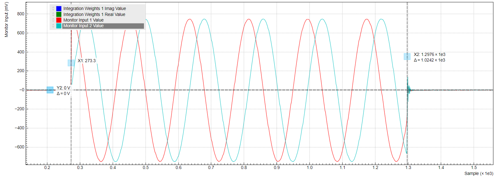
Figure 2: Dual-channel signal measured in the Quantum Analyzer Input tab

The two carrier signals correspond to the following configuration:

Signal Output 1 proportional to cos(ωt)

Signal Output 2 proportional to sin(ωt)

where ω = 2*pi*(10 MHz) is the carrier frequency. This pair of signals is then typically used as I and Q input signals of an IQ mixer with a local oscillator signal of frequency ω_LO applied to its L input. A perfect IQ mixer generates the following signal V_RF(t) at its RF port:

V_RF(t)= V_I(t)cos(ω_LOt) + V_Q(t)sin(ω_LOt)

where V_I(t) and V_Q(t) are input signals at the mixer I and Q ports. A real mixer is characterized by a certain phase imbalance θ and amplitude imbalance α, so that it effectively performs the following operation:

V_RF(t)= V_I(t)cos(ω_LOt) + V_Q(t)sin(ω_LOt+θ)α

We need to apply the following baseband signals in order to generate a signal at the lower sideband ω_LO-ω:

V_I^-(t) = cos(ωt)

V_Q^-(t) = sin(ωt-θ)/α

In order to generate a signal at the upper sideband ω_LO+ω, we need:

V_I⁺(t) = cos(ωt)

V_Q⁺(t) = -sin(ωt+θ)/α

When disregarding the mixer imperfections (θ=0, α=1), we can generate the lower sideband by connecting Signal Output 1 to the I port, and Signal Output 2 to the Q port. We can generate the upper sideband by flipping the connections between I and Q ports. This is the recommended configuration. When using AWG digital modulation in spectroscopy mode, it is not possible to correct the carriers for mixer imbalance. However, in this case this is typically not needed, since the unwanted sideband usually does not interfere with the measurement. Furthermore, the mixer imbalance depends on frequency which is an issue when either ω_LO or ω is swept. When performing qubit readout in a frequency-multiplexed fashion, mixer imbalance correction is however important in order to avoid crosstalk. It can be accounted for by modifying the carrier amplitude and phase in the programmed waveform memory.

Configure the QA Setup tab¶

In the QA Setup tab, we define the method of demodulation of the generated signals. We use the Spectroscopy mode, in which the input signals are demodulated with the in-phase and quadrature components of the internal oscillator signal. Since each readout channel delivers only a single quadrature, we will set up 2 channels to obtain both quadratures. For a full dual-phase demodulation of the two input signals, we would like to obtain the following complex amplitude:

\[\begin{equation}\tag{1} A = \int [V_1\prime(t)+iV_2\prime(t)]e^{-i\omega t}dt \end{equation}\]

V'₁(t) and V'₂(t) are the input signals after application of the deskew matrix on the left side of the QA Setup tab. Since we didn’t change the deskew matrix from its default value, which is the unit matrix, these signals are identical to the signals at the Signal Inputs, V₁(t) and V₂(t). When taking the real and imaginary part of this expression, we obtain:

\[\begin{equation}\tag{2} Re(A) = \int [V_1\prime(t)cos(\omega t) + V_2\prime(t)sin(\omega t)]dt \end{equation}\]

\[\begin{equation}\tag{3} Im(A) = \int [-V_1\prime(t)sin(\omega t) + V_2\prime(t)cos(\omega t)]dt \end{equation}\]

We configure the first two readout channels as follows such that their outputs are equal to Re(A) and Im(A), respectively:

Table 3: Settings: configure the integration
Tab	Section	#	Label	Setting / Value / State
QA Setup	Integration		Mode	Spectroscopy
QA Setup	Integration		Length	1024
QA Setup	Integration	1	Signal Input Mapping	2 → Real, 1 → Imag
QA Setup	Integration	2	Signal Input Mapping	1 → Real, 2 → Imag
QA Setup	Integration	1	Rotation	1 - 1i
QA Setup	Integration	2	Rotation	-1 - 1i

When the UHFQA is configured to operate in spectroscopy mode, a readout channel will calculate the following quantities:

\[\begin{equation}\tag{4} A_{INT} = \int [V_{REAL}\prime(t)sin(\omega t) + V_{IMAG}\prime(t)cos(\omega t)]dt, \end{equation}\]

\[\begin{equation}\tag{5} A_{ROT} = Re[\phi_{ROT} A_{INT}], \end{equation}\]

where A_INT and A_ROT are the results after integration and rotation, respectively.

Therefore, with these settings readout channel 1 will perform the following operation (note the interchanged input voltages):

\[\begin{equation}\tag{6} Re[(1-1i)\int [V_2\prime(t)cos(\omega t) + iV_1\prime(t)sin(\omega t)]dt] \end{equation}\]

Readout channel 2 will effectively perform the following operation:

\[\begin{equation}\tag{7} Re[(-1-1i)\int [V_1\prime(t)cos(\omega t) + iV_2\prime(t)sin(\omega t)]dt] \end{equation}\]

These expressions are identical to the desired quadratures Re(A) and Im(A) noted previously.

In the Quantum Analyzer Result tab, apply the settings in the table below in order to acquire an averaged measurement:

Table 4: Settings: configure the Result Logger
Tab	Sub-tab	Section	Label	Setting / Value / State
QA Result	Control	Result Wave	Source	Rotation
QA Result	Control	Result Wave	Length	2
QA Result	Control	Result Wave	Averages	32
QA Result	Control	Result Wave	Mode	Cyclic
QA Result	Control	Vertical Axis Groups	Result Wave 1 / Add Signal	click
QA Result	Control	Vertical Axis Groups	Result Wave 2 / Add Signal	click
QA Result	Control		Reset	click
QA Result	Control		Run / Stop	ON

Click on "Start/Stop" in the AWG tab in order to run the AWG. The line startQA(QA_INT_0 | QA_INT_1, true); in the AWG sequence program starts the weighted integration on the first two readout channels. 32 consecutive dual-channel pulses are acquired, integrated, averaged, and displayed.

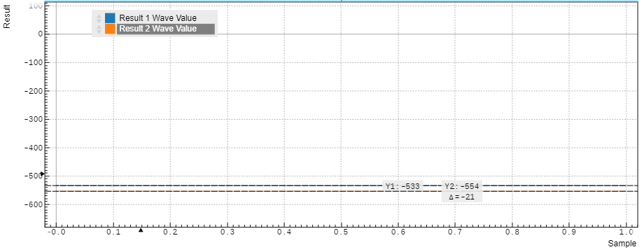
Figure 3: Measurement result at 10 MHz as displayed in the Quantum Analyzer Result tab

The data from channel 1 (blue curve) correspond to the in-phase component of the signal, the data from channel 2 (green curve) correspond to the quadrature component of the signal. For a signal with a negligible delay between generation and acquisition, we would expect this measurement to yield a zero phase, i.e., a zero quadrature component. Here, we measure an in-phase component of -533 V, and a quadrature component of -554 V. This would correspond to a normalized complex signal amplitude of (-533 - 554 i)/1024 V = 0.75 V @ -136 degrees. While the amplitude of 0.75 V corresponds well to the peak amplitude of our generated signal, but the phase is different from the naively expected value of 0 degrees. Here, this phase offset comes mainly from signal processing delays in the DAC and ADC stages, but in experiment, the length of the signal path between output and input contributes to the phase offset as well. This can normally be calibrated by changing the Rotation parameters of both measurement channels.

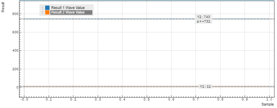
We can repeat the measurement using a much lower oscillator frequency of 10 kHz instead of 10 MHz. At this frequency, the phase offset due to signal processing delays is negligible. The following figure shows the result with an normalized in-phase component of 743/1024 V = 0.73 V, and a quadrature component of 11/1024 V = 0.01 V, corresponding well to the peak amplitude of 0.75 V at phase 0 degrees.