Weighted Integration and Result Logging¶

Note

This tutorial is applicable to all UHFQA Instruments.

Goals and Requirements¶

This tutorial explains how to analyze a pulsed signal using the weighted integration units and record the result with the Result Logger in the Quantum Analyzer Result tab.

The measurements in this tutorial can be performed using simple loop back connections.

Preparation¶

Connect the cables as illustrated below. Make sure that the UHF unit is powered on and connected by USB to your host computer or by Ethernet to your local area network (LAN) where the host computer resides. After starting LabOne the default web browser opens with the LabOne graphical user interface.

Figure 1: UHF connections for the Result Logger tutorial

The tutorial can be started with the default instrument configuration (e.g. after a power cycle) and the default user interface settings (e.g. as is after pressing F5 in the browser).

Test Signal Generation¶

First, we enable both outputs of the UHF instrument.

Table 1: Settings: observe the pulse waveform
Tab	Sub-tab	Section	#	Label	Setting / Value / State
In / Out		Signal Outputs	1	On	ON
In / Out		Signal Outputs	2	On	ON

Copy the following code into the Sequence Editor in the AWG tab.

const length = 4096;
const f_s = 1.8e9;
const f_readout = 10e6;
wave w_I = gauss(length, length/2, length/8)
             *cosine(length, 1, 0, f_readout*length/f_s);
wave w_Q = gauss(length, length/2, length/8)
             *sine(length, 1, 0, f_readout*length/f_s);

var result_length_by_2 = getUserReg(0)>>1; // We divide by two using the
                                           // bit shift operator because
                                           // each loop contains two pulses
var result_averages = getUserReg(1);

repeat (result_averages) {
  repeat (result_length_by_2) {
    playWave(w_I, w_Q);
    startQA(QA_INT_0, true);
    playZero(2*length);

    playWave(0.5*w_I, 0.5*w_Q);
    startQA(QA_INT_0, true);
    playZero(2*length);
  }
}

Upload this program to the AWG by clicking on "Save" or "To Device". The program generates a series of modulated Gaussian pulses with two alternating amplitudes. There are two nested loops: the number of pulses in the inner loop is determined by User Register 1 and would correspond to the number of points in a pulsed measurement (e.g., a Rabi flopping). The outer loop corresponds to the number of identical repetitions to be performed in order to allow averaging and is determined by User Register 2. Apply the settings in the following table to configure the AWG output as well as the User Registers.

Table 2: Settings: configure the AWG output and User Registers
Tab	Sub-tab	Section	Label	Setting / Value / State
AWG	Control		Rerun	OFF
AWG	Control	Output 1	Amplitude (FS)	1.0
AWG	Control	Output 1	Mode	Plain
AWG	Control	Output 2	Amplitude (FS)	1.0
AWG	Control	Output 2	Mode	Plain
AWG	Control	User Registers	Register 1	100 (Length)
AWG	Control	User Registers	Register 2	1 (Averages)

Configure the Integration Units¶

The AWG generates pulses with cosine and sine carrier waves at 10 MHz. In the QA Input tab, we have to define integration weights that enable demodulation of these signals at the right frequency. We choose channel 1 for this measurement.

Table 3: Settings: define the integration weights
Tab	Sub-tab	Section	Label	Setting / Value / State
QA Input	Control	Weights / Generate	Amplitude	1
QA Input	Control	Weights / Generate	Frequency	10 M
QA Input	Control	Weights / Generate	Window Length	4096
QA Input	Control	Weights / Generate	Channel	1
QA Input	Control	Weights / Generate	Set	click
QA Setup		Integration	Mode	Standard
QA Setup		Integration	Length	4096

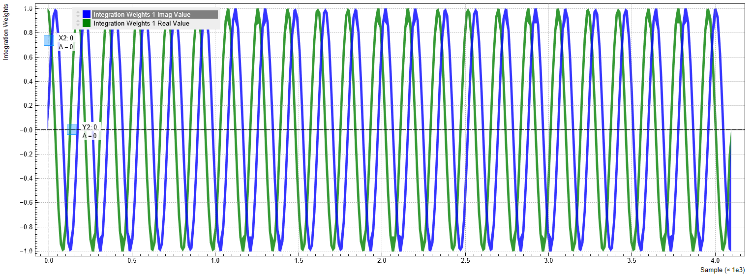
Upon clicking on Set in the QA Input tab, the sinusoid integration weights are displayed in the plot area of this tab as shown in the figure below. We denote these dimensionless weights as W_I,q(t) and W_Q,q(t), where q = 1,...,10 denotes the measurement channel, and I and Q correspond to the two signal inputs.

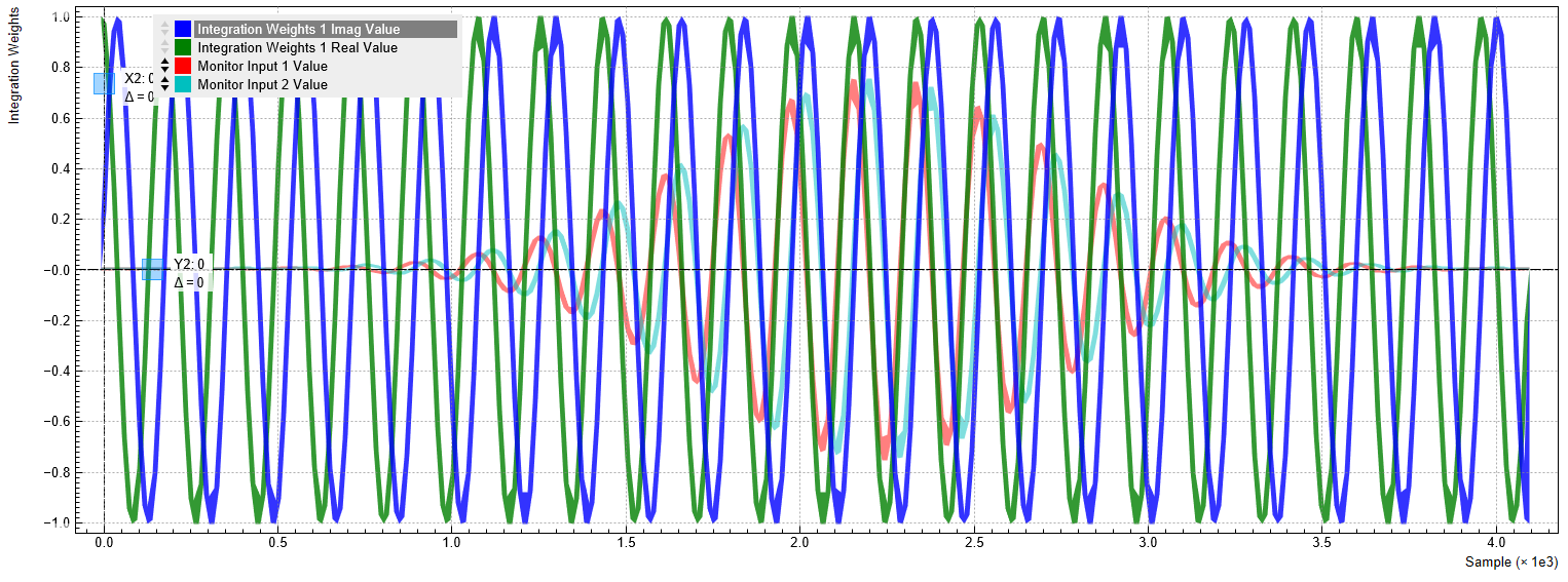
Figure 2: Integration weights as displayed in the Quantum Analyzer Input tab

We can check if the frequency of the sinusoids agree with the signal programmed in the AWG. The measurement is performed similarly as described in the previous tutorial. In the QA Input tab, set the Length to 4096 and the Averages to 64, and click on Run/Stop. Then, start the AWG by clicking on Run/Stop in the AWG tab. The peak amplitude of about 530 mV corresponds to the average between the high and low amplitude pulses generated by the AWG. We can see that the frequencies of the weights and the signal agree. An undesired delay between the signal and integration period can be compensated by using the Delay setting in the Deskew section of the QA Setup tab. Phase offsets can be compensated by directly changing the phase of the generated signal or the integration weights. Alternatively, the Rotation coefficients in the QA Setup tab allow you to rotate the signal in the complex plane after the integration. This can also be used to compensate a phase offset between signal and integration weight, but it doesn’t have an effect on the raw signal displayed in the Input Monitor.

Figure 3: Integration weights and signal as displayed in the Quantum Analyzer Input tab

In the Quantum Analyzer Input tab, apply the settings in the table below in order to conduct a measurement without averaging.

Table 4: Settings: configure the Result Logger
Tab	Sub-tab	Section	Label	Setting / Value / State
QA Result	Control	Result Wave	Source	Rotation
QA Result	Control	Result Wave	Length	100
QA Result	Control	Result Wave	Averages	1
QA Result	Control	Result Wave	Run / Stop	ON

Click on "Start/Stop" in the AWG tab in order to run the AWG. The line startQA(QA_INT_0, true); in the AWG sequence program generates a trigger to start the weighted integration. 100 consecutive dual-channel pulses are acquired, integrated, and displayed. The figure below shows the signal as displayed in the QA result tab.

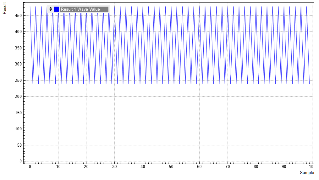
Figure 4: Measurement result as displayed in the Quantum Analyzer Result tab. The numerical values depends on the phase relation between generation and demodulation, which in turn depends on the cable length and on the Delay setting in the QA Setup tab.

These values in the graph are the integrated in-phase voltages V'_I,q after application of the Rotation coefficient of channel q. Since we left the Rotation coefficient at its default, which is 1+0i, the voltage V'_I,q is equal to the voltage V_I,q before rotation. This voltage V_I,q, along with its quadrature counterpart V_Q,q, is obtained as

\[\begin{equation}\tag{1} V_{I,q} = f_{s}\int_{0}^{T}W_{I,q}(t)V\prime_{1,q}(t)dt \end{equation}\]

\[\begin{equation}\tag{2} V_{Q,q} = f_{s}\int_{0}^{T}W_{Q,q}(t)V\prime_{2,q}(t)dt \end{equation}\]

where T is the length (in units of time) of the integration weights W_I,q(t) and W_Q,q(t), and V'_1,q(t) and V'_2,q(t) are the input signals after application of the deskew matrix accessible in the QA Setup tab, and f_s is the input sampling rate 1.8 GSa/s. Since in our case we didn’t change the deskew matrix from its default which is the unit matrix, these two signals are identical to the raw input signals on Signal Inputs 1 and 2, V_1,q(t) and V_2,q(t).

Expressed in terms of discrete-time samples n, the formula above become

\[\begin{equation}\tag{3} V_{I,q} = f_{s}\sum_{n=0}^{N-1}W_{I,q}(t)V\prime_{1,q}(t) \end{equation}\]

\[\begin{equation}\tag{4} V_{Q,q} = f_{s}\sum_{n=1}^{N-1}W_{Q,q}(t)V\prime_{2,q}(t) \end{equation}\]

where N is equal to the length (in units of samples) of the integration weights.

Note

The integrity of the data vector of the Result Logger depends on this unit receiving a number of AWG Integration triggers equal to the product of the Averages and Length settings of the Result Logger. If this condition is violated, the data of the Result Logger may get corrupted. Often, the first point of the Result vector may then contain an outlier value. Notably, the Result Logger may be driven into an invalid state ("Holdoff error") by generating an endless series of triggers, e.g. by enabling the AWG in Rerun mode.

In the given case, the integrated voltages in Figure 4 alternate between about 240 V and 480 V. This value lies in the range [– 4096×1.5 V, + 4096×1.5 V] determined by the maximum length of the integration window and the maximum input voltages. Note that the measured values depend on the phase relation between generated signal demodulation weights, which in turn depend on the cable length and on the Delay setting in the QA Setup tab.

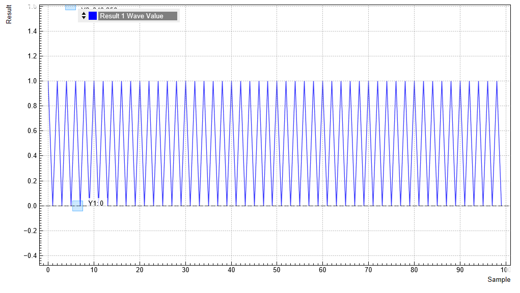
In the next step, we can apply a voltage threshold in order to discriminate the analog signal. In practice, this allows us to convert the analog readout signal in a discrete qubit state readout result. In the Thresholds section of the QA Setup tab in line 1, enter a value of 360, which lies in between the high and low readout signals in the previous measurement. Change the Source signal in the QA Result tab to Threshold, click Reset, and run again the AWG. The following table summarizes these settings.

Table 5: Settings: apply a threshold
Tab	Sub-tab	Section	#	Label	Setting / Value / State
QA Setup		Thresholds	1	Level	360
QA Result	Control	Result Wave		Source	Threshold
QA Result	Control	Result Wave		Reset	click
QA Result	Control	Result Wave		Run / Stop	ON
AWG	Control			Start / Stop	ON

Figure 5: Measurement result as measured in the Quantum Analyzer Result tab

The discretized readout results can be output with low latency as digital signal on the DIO connector on the back of the instrument. To this end, set the Digital I/O Mode to QA Result in the DIO tab. Please refer to the Digital Interface Specifications for a specification of the pin assignment.