Arbitrary Waveform Generator

Note

This tutorial is applicable to UHFQA Instruments. Where indicated, the UHF-DIG option is required in addition.

Goals and Requirements

The goal of this tutorial is to demonstrate the basic use of the AWG. We demonstrate waveform generation and playback, triggering and synchronization, carrier modulation, and sequence branching. We conclude with a list of tips for operating the AWG. To perform the measurements in this tutorial, one will require a 3rd-party programmable arbitrary waveform/function generator for trigger generation.

Preparation

Connect the cables as illustrated below. Make sure that the UHF unit is powered on and connected by USB to your host computer or by Ethernet to your local area network (LAN) where the host computer resides. After starting LabOne, the default web browser opens with the LabOne graphical user interface.

Figure 1: UHF connections for the arbitrary waveform generator tutorial

The tutorial can be started with the default instrument configuration (e.g. after a power cycle) and the default user interface settings (e.g. as is after pressing F5 in the browser).

Waveform Generation and Playback

In this tutorial we generate arbitrary signals with the AWG and visualize them with the Scope. In a first step we enable the Signal Outputs, but disable all sinusoidal signals generated by the lock-in unit by default. We also configure the Scope signal input and triggering and arm it by clicking on in the Scope. The following table summarizes the necessary settings.

Table 1: Settings: enable the output and configure the Scope

Tab	Sub-tab	Section	#	Label	Setting / Value / State
In/Out		Signal Outputs	1	Enable	ON
In/Out		Signal Outputs	2	Enable	ON
Lock-in	All	Output Amplitudes	1-8	Amp 1 Enable	OFF
Lock-in	All	Output Amplitudes	1-8	Amp 2 Enable	OFF
Scope	Control	Vertical		Channel 1	Signal Input 1
Scope	Trigger	Trigger		Enable	ON
Scope	Trigger	Trigger		Signal	Signal Input 1
Scope	Trigger	Trigger		Level	0.1 V
Scope	Control			Run/Stop	ON

Figure 2: LabOne UI: AWG tab

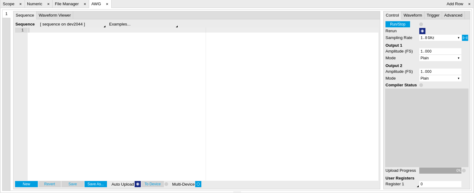
In the AWG tab, we configure both channels to output signals at the full scale (FS) in plain output mode as summarized in the following table.

Table 2: Settings: configure the AWG output

Tab	Sub-tab	Section	#	Label	Setting / Value / State
AWG	Control			Rate (Sa/s)	1.8 GHz
AWG	Control			Rerun	OFF
AWG	Control	Output 1		Amplitude (FS)	1.0
AWG	Control	Output 1		Mode	Plain
AWG	Control	Output 2		Amplitude (FS)	1.0
AWG	Control	Output 2		Mode	Plain

Operating the AWG means first of all to specify a sequence program. This can be done interactively by typing the program in the Sequence Editor window. Let’s start by typing the following code into the Sequence Editor.

wave w_gauss = 1.0*gauss(8000, 4000, 1000);
playWave(1, w_gauss);

In the first line of the program, we generate a waveform with a Gaussian shape with a length of 8000 samples and store the waveform under the name w_gauss. The peak center position 4000 and the standard deviation 1000 are both defined in units of samples. You can convert them into time by dividing by the chosen Rate (1.8 GSa/s by default). The waveform generated by the gauss function has a peak amplitude of 1. This amplitude is dimensionless and the physical signal amplitude is given by this number multiplied with the signal output range (e.g. 1.5 V). We put a scaling factor of 1.0 in place which can be replaced by any other value below 1. The code line is terminated by a semicolon according to C conventions. In the second line, the generated waveform w_gauss is played on AWG Output 1.

Note

For this tutorial, we will keep the description of the Sequencer commands short. You can find the full specification of the LabOne Sequencer language in LabOne Sequence Programming

Note

The AWG has a waveform granularity of 16 samples. It’s recommended to use waveform lengths that are multiples of 16, e.g. 8000 like in this example, to avoid having ill-defined samples between successively played waveforms. Other waveform lengths are allowed, though.

If we now click on , the program gets compiled. This means the program is translated into instructions for the LabOne Sequencer on the UHF instrument, see AWG Tab. If no error occurs (due to wrong program syntax, for example), the Status LED lights up green, and the resulting program as well as the waveform data is written to the instrument memory. If an error or warning occurs, messages in the Status field will help in debugging the program. If we now have a look at the Waveform sub-tab, we see that our Gaussian waveform appeared in the list. The Memory Usage field at the bottom of the Waveform sub-tab shows what fraction of the instrument memory is filled by the waveform data. The Waveform viewer sub-tab allows you to graphically display the currently marked waveform in the list.

By clicking on with Rerun disabled, we have the AWG execute our program once. Since we have armed the Scope previously with a suitable trigger level, it has captured our Gaussian pulse with a FWHM of about 1.33 μs as shown in Figure 3.

Figure 3: Gaussian pulse as generated by the AWG and captured by the LabOne Scope

The LabOne Sequencer language contains various control structures. The basic functionality is to play back a waveform several times. In the following example, all the code within the curly brackets '{...}' is repeated 5 times. Upon clicking and you should observe 5 short Gaussian pulses in a new scope shot, see Figure 4 .

wave w_gauss = 1.0 * gauss(640, 320, 50);

repeat (5) {
  playWave(1, w_gauss);
}

Figure 4: Burst of Gaussian pulses generated by the AWG and captured by the LabOne Scope

In order to generate more complex waveforms, the LabOne Sequencer programming language offers a rich toolset for waveform editing. On the basis of a selection of standard waveform generation functions, waveforms can be added, multiplied, scaled, concatenated, and truncated. It’s also possible to use compile-time evaluated loops to generate pulse series with systematic parameter variations – see LabOne Sequence Programming for more precise information. In the following code example, we make use of these tools to generate a pulse with a smooth rising edge, a flat plateau, and a smooth falling edge. We use the cut function to cut a waveform at defined sample indices, the rect function to generate a waveform with constant level 1.0 and length 320, and the join function to concatenate three (or arbitrarily many) waveforms.

wave w_gauss = gauss(640, 320, 50);
wave w_rise = cut(w_gauss, 0, 319);
wave w_fall = cut(w_gauss, 320, 639);
wave w_flat = rect(320, 1.0);

wave w_pulse = join(w_rise, w_flat, w_fall);

while (true) {
  playWave(1, w_pulse);
}

Note that we replaced the finite repetition by an infinite repetition by using a while loop. Loops can be nested in order to generate complex playback routines. The Rerun button in the Control sub-tab will simply cause the entire AWG program to be restarted automatically. This is a simple alternative for creating loops, however, unlike the while loop the Rerun method does not allow back-to-back waveform playback and comes with a certain timing jitter. The output generated by the program above is shown in Figure 5.

Figure 5: Infinite pulse series generated by the AWG and captured by the LabOne Scope

One pitfall when using loops has to do with the nature of the playWave and related commands. This command initiates the waveform playback, but during the playback the sequencer will start to execute the next command on his list. This is useful as it allows you to execute commands during playback. In a loop, it means the sequencer can jump back to the beginning of the loop while the waveform is still being played. You can easily change this behavior by adding waitWave as the last command in the loop.

As programs get longer, it becomes useful to store and recall them. Clicking on allows you to store the present program under a newly chosen file name. Clicking on then saves your program to the file name displayed at the top of the editor. As you begin to work on sequence programs more regularly, it’s worth expanding your repertoire by some of the editor keyboard shortcuts listed in Sequence Editor Keyboard Shortcuts.

It’s also possible to iterate over the samples of a waveform array and calculate each one of them in a loop over a compile-time variable cvar. This often allows to go beyond the possibilities of using the predefined waveform generation function, particularly when using nested formulas of elementary functions like in the following example. The waveform array needs to be pre-allocated e.g. using the instruction zeros.

const N = 1024;
const width = 100;
const position = N/2;
const f_start = 0.1;
const f_stop = 0.2;
cvar i;
wave w_array = zeros(N);
for (i = 0; i < N; i++) {
  w_array[i] = sin(10/(cosh((i-position)/width)));
}

playWave(w_array);

Should you require more customization than what is offered by the LabOne AWG Sequencer language, you can import any waveform from a comma-separated value (CSV) file. The CSV file should contain floating-point values in the range from –1.0 to +1.0 and contain one or several columns, corresponding to the number of channels. As an example, the following could be the contents of a file wave_file.csv specifying a dual-channel wave with a length of 16 samples:

  -1.0   0.0
  -0.8   0.0
  -0.7   0.1
  -0.5   0.2
  -0.2   0.3
  -0.1   0.2
 0.1   0.0
 0.2    -0.1
 0.7    -0.3
 1.0    -0.2
 0.9    -0.3
 0.8    -0.2
 0.4    -0.1
 0.0    -0.1
  -0.5    -0.1
  -0.8   0.0

Store the file in the location of C:\Users\<user name>\Documents\Zurich Instruments\LabOne\WebServer\awg\waves\wave_file.csv under Windows or ~/Zurich Instruments/LabOne/WebServer/awg/waves/wave_file.csv under Linux. In the sequence program you can then play back the wave by referring to the file name without extension:

playWave("wave_file");

If you prefer, you can also store it in a wave data type first and give it a new name:

wave w = "wave_file";
playWave(w);

The external wave file can have arbitrary content, but consider that the final signal will pass through the 600 MHz low-pass filter of the instrument. This means that signal components exceeding the filter bandwidth are not reproduced exactly as suggested for example by looking at a plot of the waveform data. In particular, this concerns sharp transitions from one sample to the next.

In order to obtain digital marker data (see below) from a file, specify a second wave file with integer instead of floating-point values. The marker bits are encoded in the binary representation of the integer (i.e., integer 1 corresponds to the first marker high, 2 corresponds to the second marker high, and 3 corresponds to both bits high). Later in the program add up the analog and the marker waveforms. For instance, if the floating-point analog data are contained in wave_file_analog.csv and the integer marker data in wave_file_digital.csv, the following code can be used to combine and play them.

wave w_analog  = "wave_file_analog";
wave w_digital = "wave_file_digital";
wave w = w_analog + w_digital;
playWave(w);

As an alternative to specifying analog data as floating-point values in one file, and marker data as integer values in a second file, both may be combined into one file containing integer values that correspond to the raw data format of the instrument. The integer values in that file should be 16-bit unsigned integers with the two least significant bits being the markers. The values are mapped to 0 ⇒ -FS, 65535 ⇒ +FS, with FS equal to the full scale.

Triggering and Synchronization

Now we have a look at the triggering functionality of the AWG. In this section we will explain how to deal with the most important use cases:

• Triggering the AWG with an external TTL signal
• Generating a TTL signal with the AWG to trigger an external device
• Control the AWG repetition rate by an internal oscillator

We will simulate these situations with on-board means of the UHF instrument for the sake of simplicity, but the inclusion of external equipment is straightforward in practice.

The AWG’s trigger channels can be freely linked to a variety of connectors, such as the bidirectional Trigger connectors on the front panel, and other functional units inside the instrument, such as the Scope or the Qubit Measurement Unit . This freedom of configuration is enabled by the Cross-Domain Trigger feature and enables triggering.

Triggering the AWG

In this section we show how to trigger the AWG with an external TTL signal. Please use a third-party instrument, such as a function generator, to generate a square wave with 300 kHz frequency and connect this signal to the Trigger Input 1 on the front panel.

The AWG has 4 trigger input channels. As discussed, these are not directly associated with physical device inputs but can be freely configured to probe a variety of internal or external signals. Here, we link the AWG Digital Trigger 1 to the physical Trigger 1 connector.

Table 3: Settings: configure the AWG analog trigger input

Tab	Sub-tab	Section	#	Label	Setting / Value / State
AWG	Trigger	Digital Trigger 1		Signal	Trig Input 1
AWG	Trigger	Digital Trigger 1		Slope	Rise

Finally, we modify our last AWG program by including a waitDigTrigger command just before the playWave command. The result is that upon every repetition inside the infinite while loop, the AWG will wait for a rising flank on Trigger input 1.

wave w_gauss = gauss(640, 320, 50);
wave w_rise  = cut(w_gauss, 0, 319);
wave w_fall  = cut(w_gauss, 320, 639);
wave w_flat  = rect(320, 1.0);

wave w_pulse = join(w_rise, w_flat, w_fall);

while (true) {
  waitDigTrigger(1, 1);
  playWave(1, w_pulse);
}

Compile and run the above program. Note that this and other programming examples are available directly from a drop-down menu on top of the Sequence Editor. Figure 6 shows the pulse series as seen in the Scope: the pulses are now spaced by the oscillator period of about 3.3 μs, unlike previously when the period was determined by the length of the waveform w_pulse. Try changing the frequency of the external trigger signal , or unplugging the trigger cable, to observe the immediate effect on the signal.

Figure 6: Externally triggered pulse series generated by the AWG and captured by the LabOne Scope

Generating Triggers with the AWG

There are two ways of generating trigger output signals with the AWG: as markers, or through sequencer commands.

The method using markers is recommended when precise timing is required, and/or complicated serial bit patterns need to be played on the trigger outputs. Marker bits are part of every waveform which is an array of 16-bit words: 14 bits of each word represent the analog waveform data, and the remaining 2 bits represent two digital marker channels. Upon playback, a digital signal with sample-precise alignment with the analog output is generated.

The method using a sequencer command is simpler, but the timing control is less flexible than when using markers. It is useful for instance to generate a single trigger signal at the start of an AWG program.

Table 4: Comparison: AWG markers and triggers

	Marker	Trigger
Implementation	Part of waveform	Sequencer command
Timing control	High	Low
Generation of serial bit patterns	Yes	No
Cross-device synchronization	Yes	Yes

Let us first demonstrate the use of markers. In the following code example we first generate a Gaussian pulse again. The so generated wave does include marker bits – they are simply set to zero by default. We use the marker function to assign the desired non-zero marker bits to the wave. The marker function takes two arguments, the first is the length of the wave, the second is the marker configuration in binary encoding: the value 0 stands for a both marker bits low, the values 1, 2, and 3 stand for the first, the second, and both marker bits high, respectively. We use this to construct the wave called w_marker.

const marker_pos = 3000;

wave w_gauss  = gauss(8000, 4000, 1000);
wave w_left   = marker(marker_pos, 0);
wave w_right  = marker(8000-marker_pos, 1);
wave w_marker = join(w_left, w_right);
wave w_gauss_marker = w_gauss + w_marker;

playWave(1, w_gauss_marker);

The waveform addition with the '+' operator adds up analog waveform data but also combines marker data. The wave w_gauss contains zero marker data, whereas the wave w_marker contains zero analog data. Consequentially the wave called w_gauss_marker contains the merged analog and marker data. We use the integer constant marker_pos to determine the point where the first marker bit flips from 0 to 1 somewhere in the middle of the Gaussian pulse.

Note

The add function and the '+' operator combine marker bits by a logical OR operation. This means combining 0 and 1 yields 1, and combining 1 and 1 yields 1 as well.

The following table summarizes the settings to apply in order to output marker 1 on Trigger 2, and to configure the scope to trigger on Trigger 1.

Table 5: Settings: configure the AWG marker output and scope trigger

Tab	Sub-tab	Section	#	Label	Setting / Value / State
DIO		Output	2	Signal	AWG Marker 1
DIO		Output	2	Drive	ON
Scope	Trigger	Trigger		Signal	Trig Input 1

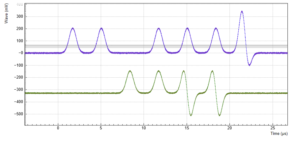
Figure 7 shows the AWG signal captured by the Scope. The green curve shows the second Scope channel (requires UHF-DIG option) configured to display the Trigger Input 1 signal. Try changing the marker_pos constant and re-running the sequence program to observe the effect on the temporal alignment of the Gaussian pulse.

Figure 7: Pulse and marker signal generated by the AWG and captured by the LabOne Scope (dual-channel Scope operation requires UHF-DIG option)

Let us now demonstrate the use of sequencer commands to generate a trigger signal. Copy and paste the following code example into the Sequence Editor.

wave w_gauss = gauss(8000, 4000, 1000);

setTrigger(1);
playWave(1, w_gauss);
waitWave();
setTrigger(0);

The setTrigger function takes a single argument encoding the four AWG Trigger output states in binary form – the integer number 1 corresponds to a configuration of 0/0/0/1 for the trigger outputs 4/3/2/1. The binary integer notation of the form 0b0000 is useful for this purpose – e.g. setTrigger(0b0011) will set trigger outputs 1 and 2 to 1, and trigger outputs 3 and 4 to 0. We included a waitWave command after the playWave command. It ensures that the subsequent setTrigger command is executed only after the Gaussian wave has finished playing, and not during waveform playback.

We reconfigure the Trigger 2 connector such that it outputs the AWG Trigger 1, instead of the AWG Marker 1. The rest of the settings can stay unchanged.

Table 6: Settings: configure the AWG trigger output

Tab	Sub-tab	Section	#	Label	Setting / Value / State
DIO		Output	2	Signal	AWG Trigger 1

Figure 8 shows the AWG signal captured by the Scope. This looks very similar to Figure 7 in fact. With this method, we’re less flexible in choosing the trigger time, as the rising trigger edge will always be at the beginning of the waveform. But we don’t have to bother about assigning the marker bits to the waveform.

Figure 8: Pulse and trigger signal generated by the AWG and captured by the LabOne Scope (dual-channel Scope operation requires UHF-DIG option)

Signal Output Assignment

In addition to the single-channel and dual-channel playback used up to now, there are more options for the channel assignment. The playWave command can be used with different combinations of arguments: with one wave type argument or with two, with a const type integer number specifying the signal output or without. These different combinations of arguments allow the user to independently control the AWG outputs (the digital signal sources inside the instrument) and the place where their signal is routed to (the signal outputs on the front panel). The AWG outputs are represented in the AWG tab, whereas the signal outputs are represented in the In / Out tab .

The playWave command always assigns the first wave argument to the AWG output 1, and the second one (if it’s provided) to the AWG output 2. Each of the wave arguments can optionally be preceded by an integer argument of type const which specifies the associated signal output. E.g., playWave(2, w_gauss) will play the wave w_gauss on Signal Output 2.

It’s possible to route a single AWG Output to both Signal Outputs at the same time by specifying two integer arguments per wave argument as in playWave(1, 2, w_gauss). This can for example be used to optimize waveform memory. Another option is to add up two AWG Outputs on one Signal Output by using twice the same integer argument as in playWave(1, w_gauss, 1, w_drag). The following sequence program contains a number of examples for these configurations. Figure 9 shows the dual-channel signal generated with this program and measured with the LabOne Scope.

wave w_gauss = gauss(640, 320, 50);

while (true) {
  waitDemodOscPhase(8);
  playWave(1, w_gauss);
}

Note

Tricky examples are commands like playWave(2, w_gauss) that generate a signal on Signal Output 2, but use the AWG output 1. This means that the relevant Mode and Amplitude (FS) settings are in the section Output 1 of the AWG tab, not in the section Output 2.

Figure 9: Dual-channel signal generated by the AWG and captured by the LabOne Scope (dual-channel Scope operation requires UHF-DIG option). The vertical scales of the two signals have been offset, see

Four-channel Aux Output

For applications requiring more channels and/or higher voltages, the UHF-AWG can generate signals on the auxiliary outputs of the UHF instrument. To this end the AWG resources for one fast channel (1.8 GSa/s) can be reallocated so as to generate four independent signals at 14 MSa/s and 16 bit resolution in a ±10 V range.

In the sequence program, the functionality is available through the playAuxWave function. The function requires four waveforms of equal length as arguments.

We configure the multi-purpose Auxiliary Outputs for AWG signal generation by setting the Auxiliary Output Signal to AWG in the Auxiliary tab. Each Auxiliary Output corresponds to one of the four rows in the tab. The Channel setting allows you to route one of the four AWG Outputs (the four waveforms of the playAuxWave command) to the given Auxiliary Output. Typically for the first row the Channel is set to 1, for the second row to 2, and so forth.

We intend to monitor the individual Auxiliary signals with the Scope on Signal Input 1. Before making the corresponding BNC connections, it’s good practice to adjust the Auxiliary Output Lower and Upper Limits in order to prevent damage to the Signal Input. You can use the Scale and the Offset setting in order to modify the signal.

The Auxiliary Outputs have a much lower analog bandwidth than the Signal Outputs. It is therefore necessary to work at a sampling rate of 14 MSa/s or less. In order to combine slow Auxiliary Output signals with fast signals on the Signal Outputs, it’s useful to set the sampling rate for every individual waveform play command. In the following example, we first play four waveforms in parallel on the Auxiliary Outputs at reduced sampling rate, and then one waveform on the Signal Output 2 at full sampling rate.

// Sampling rate of the system, adjust accordingly if the rate is reduced
const FS = 1800e6;
// Frequency of the 'sine' in the SINC waveform
const F_SINC = 42e6;

// Generate the four-channel auxiliary output waveform
wave aux_ch1 =  1.0*gauss(8000, 4000, 1000);
wave aux_ch2 =  0.5*gauss(8000, 4000, 1000);
wave aux_ch3 = -0.5*gauss(8000, 4000, 1000);
wave aux_ch4 = -1.0*gauss(8000, 4000, 1000);

// Generate a waveform to be played on Signal Output 2
wave w_sinc = sinc(8000, 4000, FS/F_SINC);

while (true) {
  // play the four Aux Output channels at reduced rate
  playAuxWave(aux_ch1, aux_ch2, aux_ch3, aux_ch4, AWG_RATE_14MHZ);
  // play a wave on Signal Output 2
  playWave(w_sinc, AWG_RATE_1800MHZ);
}

The following table summarizes the settings to be made for this example.

Table 7: Settings: configure the AWG for generating signals on the Auxiliary

Tab	Sub-tab	Section	#	Label	Setting / Value / State
AWG	Control	Output 1/2		Mode	Plain
Auxiliary		Aux Output	1-4	Lower/Upper Limit	–1.5 V/+1.5 V
Auxiliary		Aux Output	1-4	Signal	AWG
Auxiliary		Aux Output	1	Channel	1
Auxiliary		Aux Output	2	Channel	2
Auxiliary		Aux Output	3	Channel	3
Auxiliary		Aux Output	4	Channel	4

Outputs

Note

The four-channel AWG mode features a sample hold functionality: the output voltage of the last sample of a waveform remains fixed after the waveform playback is over. This can be used to control the output voltage between pulses.

Debugging Sequencer Programs

When generating fast signals and observing them with the LabOne Scope, in some configurations you may observe timing jitter or unexpected delays in the generated signal. There are two main reasons for that. The first reason is linked to the AWG’s memory architecture, which is based on a main memory and a cache memory. Waveform data stored in the main memory (128 MSa per channel) must be copied to the cache memory (32 kSa per channel) prior to playback. The bandwidth available for this data transfer is less than that required by the AWG for dual-channel operation at 1.8 GSa/s. Therefore, if the AWG is configured to play waveforms longer than what fits in the cache memory in dual-channel mode at 1.8 GSa/s, interruptions in the generated signal may be observed. The second reason is connected to the AWG compiler concept explained in Description. When a program in the Sequence Editor is compiled into machine code that can be executed by the Sequencer hardware, single lines of code may be expanded into several machine instructions. Each instruction requires one clock cycle (4.44 ns) for execution. Therefore, the final timing of the generated waveform may not always be completely apart from looking solely at the high-level sequencer program. The compiled program, which defines the actual timing, is displayed in the Advanced sub-tab.

Please take the following tips into consideration when operating the UHF-AWG. They should help you prevent and solve timing problems.

• The Scope and the AWG share the same memory, which means that operating them together at high sampling rates affects the performance of both of them. Note that this is only a concern when the AWG is playing back waveforms that are too large to fit in the cache memory. If this is the case it may prove difficult to visualize the generated AWG signal using the LabOne Scope. One option for visualizing such long waveforms is to reduce the sampling rate of both the AWG and the Scope to 225 MHz, which allows both the AWG and the Scope to operate in dual-channel mode simultaneously. The overall shape of the generate AWG signal can then be visualized and evaluated. The sampling rate of the AWG can then be increased once you are satisfied with the shape of the generated signals.
• Minimize waveform memory (1): use the possibility to vary the sample rate during playback. The playWave command (and related commands) accept a sampling rate parameter, which means slow and fast signal components can be played at different rates.
• Minimize waveform memory (2): take advantage of the amplitude modulation mode in order to generate signals at the full bandwidth, but with reduced envelope sampling rate.
• Minimize waveform memory (3): in four-channel (Auxiliary Output) mode, the signal amplitude of the last sample after a waveform playback is held. This eliminates the need for long waveforms with constant amplitude, e.g. on a pulse plateau.
• Check the occupied waveform cache memory in the Waveform sub-tab. If you stay below 100%, the performance is best and there is no interference with the LabOne Scope.
• Take advantage of the AWG state signals available on the Trigger outputs. In the DIO tab you can select from a number of options for outputting the AWG state as TTL signals, such as "fetching", or "playing". Monitoring these signals on a scope can help in understanding the AWG timing.
• When possible, use the repeat loop instead of the for and while loops. The for and while loops evaluate and compare run-time variables, which makes them slower to execute in comparison to the repeat loop.
• Fill up sequencer waiting time with useful commands. Placing commands and run-time variable operations just before a wait command (and related commands) in the sequence program means they will be executed when the sequencer has time.
• When you need sample-precise timing between analog and digital output signals, use the AWG Markers rather than the AWG Triggers or the DIO outputs.
• When using the four-channel Auxiliary Output mode, be aware that the timing between Signal Output and Aux outputs is not well-defined. Use a scope to adjust inter-channel delays.
• Be aware that the sequencer instruction memory is also segmented into a cache memory and main memory. Very long sequence programs therefore require fetching operations, which costs some time. You can read the memory usage in the Advanced sub-tab.