This chapter contains reference documentation for the settings and
measurement data available on UHFQA Instruments. Whilst
Functional Description LabOne User Interface
describes many of these settings in terms of the features available in
the LabOne User Interface, this chapter describes them on the device
level and provides a hierarchically organized and comprehensive list of
device functionality.
Since these settings and data streams may be written and read using the
LabOne APIs (Application Programming Interfaces) this chapter is of
particular interest to users who would like to perform measurements
programmatically via LabVIEW, Python, MATLAB, .NET or C.
Please see:
Introduction for an introduction of how the
instrument’s settings and measurement data are organized
hierarchically in the Data Server’s so-called "Node Tree".
Reference Node Documentation for a reference list of
the settings and measurement data available on UHFQA Instruments,
organized by branch in the Node Tree.
This chapter provides an overview of how an instrument’s configuration
and output is organized by the Data Server.
All communication with an instrument occurs via the Data Server program
the instrument is connected to (see LabOne Software
Architecture
for an overview of LabOne’s software components). Although the
instrument’s settings are stored locally on the device, it is the Data
Server’s task to ensure it maintains the values of the current settings
and makes these settings (and any subscribed data) available to all its
current clients. A client may be the LabOne User Interface or a user’s
own program implemented using one of the LabOne Application Programming
Interfaces, e.g., Python.
The instrument’s settings and data are organized by the Data Server in a
file-system-like hierarchical structure called the node tree. When an
instrument is connected to a Data Server, its device ID becomes a
top-level branch in the Data Server’s node tree. The features of the
instrument are organized as branches underneath the top-level device
branch and the individual instrument settings are leaves of these
branches.
For example, the auxiliary outputs of the instrument with device ID
"dev2006" are located in the tree in the branch:
/dev1000/auxouts/
In turn, each individual auxiliary output channel has its own branch
underneath the "AUXOUTS" branch.
Whilst the auxiliary outputs and other channels are labelled on the
instrument’s panels and the User Interface using 1-based indexing, the
Data Server’s node tree uses 0-based indexing. Individual settings (and
data) of an auxiliary output are available as leaves underneath the
corresponding channel’s branch:
These are all individual node paths in the node tree; the lowest-level
nodes which represent a single instrument setting or data stream.
Whether the node is an instrument setting or data-stream and which type
of data it contains or provides is well-defined and documented on a
per-node basis in the Reference Node Documentation section in the
relevant instrument-specific user manual. The different properties and
types are explained in Node Properties and Data Types
.
For instrument settings, a Data Server client modifies the node’s value
by specifying the appropriate path and a value to the Data Server as a
(path, value) pair. When an instrument’s setting is changed in the
LabOne User Interface, the path and the value of the node that was
changed are displayed in the Status Bar in the bottom of the Window.
This is described in more detail in Exploring the Node Tree.
Module Parameters
LabOne Core Modules, such as the Sweeper, also use a similar tree-like
structure to organize their parameters. Please note, however, that
module nodes are not visible in the Data Server’s node tree; they are
local to the instance of the module created in a LabOne client and are
not synchronized between clients.
A node may have one or more of the following properties:
Read
Data can be read from the node.
Write
Data can be written to the node.
Setting
The node corresponds to a writable instrument configuration. The data of these nodes are persisted in snapshots of the instrument and stored in the LabOne XML settings files.
Streaming
A node with the read attribute that provides instrument data, typically at a user-configured rate. The data is usually a more complex data type, for example demodulator data is returned as ZIDemodSample. A full list of streaming nodes is available in the Programming Manual in the Chapter Instrument Communication. Their availability depends on the device class (e.g. MF) and the option set installed on the device.
A node may contain data of the following types:
Integer
Integer data.
Double
Double precision floating point data.
String
A string array.
Integer (enumerated)
As for Integer, but the node only allows certain values.
Composite data type
For example, ZIDemodSample. These custom data types are structures whose fields contain the instrument output, a timestamp and other relevant instrument settings such as the demodulator oscillator frequency. Documentation of custom data types is available in
A convenient method to learn which node is responsible for a specific
instrument setting is to check the Command Log history in the bottom of
the LabOne User Interface. The command in the Status Bar gets updated
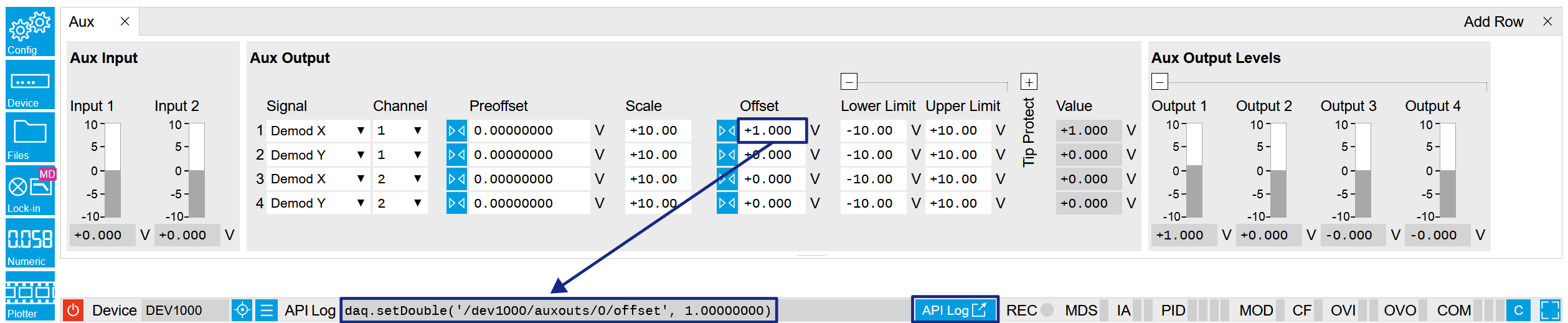
every time a configuration change is made. Figure 1 shows how the equivalent MATLAB
command is displayed after modifying the value of the auxiliary output
1’s offset. The format of the LabOne UI’s command history can be
configured in the Config Tab (MATLAB, Python and .NET are available).
The entire history generated in the current UI session can be viewed by
clicking the "Show Log" button.
Figure 1: When a device’s configuration is modified in the LabOne User Interface, the Status Bar displays the equivalent command to perform the same configuration via a LabOne programming interface. Here, the MATLAB code to modify auxiliary output 1’s offset value is provided. When "Show Log" is clicked the entire configuration history is displayed in a new browser tab.
In a LabOne Programming Interface
A list of nodes (under a specific branch) can be requested from the Data
Server in an API client using the listNodes command (MATLAB, Python,
.NET) or ziAPIListNodes() function (C API). Please see each API’s
command reference for more help using the listNodes command. To obtain
a list of all the nodes that provide data from an instrument at a high
rate, so-called streaming nodes, the streamingonly flag can be
provided to listNodes. More information on data streaming and
streaming nodes is available in the LabOne Programming Manual.
The detailed descriptions of nodes that is provided in
Reference Node Documentation is accessible directly in the LabOne MATLAB or Python
programming interfaces using the "help" command. The help command is
daq.help(path) in Python and ziDAQ('help', path) in MATLAB. The
command returns a description of the instrument node including access
properties, data type, units and available options. The "help" command
also handles wildcards to return a detailed description of all nodes
matching the path. An example is provided below.
daq=zhinst.core.ziDAQServer('localhost',8004,6)daq.help('/dev2006/auxouts/0/offset')# Out:# /dev1000/auxouts/0/offset## Add the specified offset voltage to the signal after scaling. Auxiliary Output# Value = (Signal+Preoffset)*Scale + Offset# Properties: Read, Write, Setting# Type: Double# Unit: V
The Data Server has nodes in the node tree available under the top-level
/ZI/ branch. These nodes give information about the version and state of
the Data Server the client is connected to. For example, the nodes:
/ZI/ABOUT/VERSION
/ZI/ABOUT/REVISION
are read-only nodes that contain information about the release version
and revision of the Data Server. The nodes under the /ZI/DEVICES/ list
which devices are connected, discoverable and visible to the Data
Server.
The nodes:
/ZI/CONFIG/OPEN
/ZI/CONFIG/PORT
are settings nodes that can be used to configure which port the Data
Server listens to for incoming client connections and whether it may
accept connections from clients on hosts other than the localhost.
Nodes that are of particular use to programmers are:
/ZI/DEBUG/LOGPATH - the location of the Data Server’s log in the PC’s
file system,
/ZI/DEBUG/LEVEL - the current log-level of the Data Server
(configurable; has the Write attribute),
/ZI/DEBUG/LOG - the last Data Server log entries as a string array.
The Global nodes of the LabOne Data Server are listed in the Instrument Communication
chapter of the LabOne Programming Manual
Defines the number of samples on the input to average as a power of two. Possible values are in the range [0, 16]. A value of 0 corresponds to the sampling rate of the auxiliary input's ADC.
Voltage measured at the Auxiliary Input after averaging. The data rate depends on the averaging value. Note, if the instrument has demodulator functionality, the auxiliary input values are available as fields in a demodulator sample and are aligned by timestamp with the demodulator output.
Voltage measured at the Auxiliary Input after averaging. The value of this node is updated at a low rate (50 Hz); the streaming node auxins/n/sample is updated at a high rate defined by the averaging.
"normal": Normal: Logger starts with the AWG and overwrites old values as soon as the memory limit of 1024 entries is reached.
1
"timestamp": Timestamp-triggered: Logger starts with the AWG, waits for the first valid trigger, and only starts recording data after the time specified by the starttimestamp. Recording stops as soon as the memory limit of 1024 entries is reached.
Status of the sequencer on the instrument. Bit 0: sequencer is running; Bit 1: reserved; Bit 2: sequencer is waiting for a trigger to arrive; Bit 3: sequencer is not ready; Bit 4: sequencer is waiting for synchronization with other channels.
Node used by the sweeper module for fast index sweeps. When selected as sweep grid the sweeper module will switch into a fast index based scan mode. This mode can be up to 1000 times faster than conventional node sweeps. The sequencer program must support this functionality. See section 'AWG Index Sweep' of the UHF user manual for more information.
AWG sampling rate. The numeric values are rounded for display purposes. The exact values are equal to the base sampling rate (1.8 GHz) divided by 2^n, where n is the node value. This value is used by default and can be overridden in the Sequence program.
Defines the voltage the source signal must deviate from the trigger level before the trigger is rearmed again. Set to 0 to turn it off. The sign is defined by the Edge setting.
Selects the mode to define the hysteresis strength. The relative mode will work best over the full input range as long as the analog input signal does not suffer from excessive noise.
0
"absolute": Selects absolute hysteresis (V).
1
"relative": Selects a hysteresis relative to the adjusted full scale signal input range (%).
JSON-formatted string containing a dictionary of various properties of the current waveform: name, filename, function, channels, marker bits, length, timestamp.
Amount of the used waveform data relative to the device cache memory. The cache memory provides space for 32 kSa (32'768 Sa) per-channel of waveform data. Memory Usage over 100% means that waveforms must be loaded from the main memory of 64 MSa (67'108'864 Sa) per-channel during playback, which can lead to delays.
The waveform data in the instrument's native format for the given playWave waveform index. This node will not work with subscribe as it does not push updates. For short vectors get may be used. For long vectors (causing get to time out) getAsEvent and poll can be used. The index of the waveform to be replaced can be determined using the Waveform sub-tab in the AWG tab of the LabOne User Interface.
When on (1), the corresponding 8-bit bus is in output mode. When off (0), it is in input mode. Bit 0 corresponds to the least significant byte. For example, the value 1 drives the least significant byte, the value 8 drives the most significant byte.
The DIO is internally clocked with a frequency of 56.25 MHz.
1
"external": The DIO is externally clocked with a clock signal connected to DIO Pin 68. The available range is from 1 Hz up to the internal clock frequency.
2
"internal": The DIO is internally clocked with a frequency of 50 MHz.
Transformation coefficients for each channel as a 10×10 matrix. The values are defined as floating point numbers. In hardware, the coefficients are implemented as 17-bit signed integers.
Integration time of all weighted integration units specified in units of samples. A maximum of 4096 samples can be integrated, which corresponds to 2.3 µs.
The weight functions to be applied on the imaginary part of the input signal. The weights are written as vectors. In the hardware the weights are implemented as 17-bit integers.
The weight functions to be applied on the real part of the input signal. The weights are written as vectors. In the hardware the weights are implemented as 17-bit integers.
log2 of the number of averages to perform, i.e. 0 means no averaging, 1 means 2 values are averaged, etc. Maximum setting is 15 meaning 2^15 values are averaged.
log2 of the number of averages to perform, i.e. 0 means no averaging, 1 means 2 values are averaged, etc. Maximum setting is 15 meaning 2^15 values are averaged.
Number of state errors measured for this channel. A state error occurs when there is a discrepancy between the measured state of this channel and the state that is predicted based on the configured state table.
Defines the state table. The node has one entry for each possible state, i.e. 32 entries in case of five readout channels. The value of each entry defines the expected next state as a simple bit mask mapped to an unsigned integer.
Lower limit of the scope full scale range. For demodulator, PID, Boxcar, and AU signals the limit should be adjusted so that the signal covers the specified range to achieve optimal resolution.
Upper limit of the scope full scale range. For demodulator, PID, Boxcar, and AU signals the limit should be adjusted so that the signal covers the specified range to achieve optimal resolution.
Specifies the number of segments to be recorded in device memory. The maximum scope shot size is given by the available memory divided by the number of segments. This functionality requires the DIG option.
Enable segmented scope recording. This allows for full bandwidth recording of scope shots with a minimum dead time between individual shots. This functionality requires the DIG option.
Enable scope streaming for the specified channel. This allows for continuous recording of scope data on the plotter and streaming to disk. Note: scope streaming requires the DIG option.
Streaming Rate of the scope channels. The streaming rate can be adjusted independent from the scope sampling rate. The maximum rate depends on the interface used for transfer. Note: scope streaming requires the DIG option.
Trigger position relative to reference. A positive delay results in less data being acquired before the trigger point, a negative delay results in more data being acquired before the trigger point.
Defines the trigger event number that will trigger the next recording after a recording event. A value of '1' will start a recording for each trigger event.
Defines the voltage the source signal must deviate from the trigger level before the trigger is rearmed again. Set to 0 to turn it off. The sign is defined by the Edge setting.
Selects the mode to define the hysteresis strength. The relative mode will work best over the full input range as long as the analog input signal does not suffer from excessive noise.
0
"absolute": Selects absolute hysteresis.
1
"relative": Selects a hysteresis relative to the adjusted full scale signal input range.
Sets on which slope of the trigger signal the scope should trigger. This setting is synchronized with the settings done in the /TRIGFALLING and /TRIGRISING nodes.
0
"none": None
1
"rising": Rising edge triggered.
2
"falling": Falling edge triggered.
3
"both": Triggers on both the rising and falling edge.
Switch input mode between normal (OFF), inverted, and differential. The differential modes are implemented digitally and are not suited for analog common-mode rejection. When using the differential modes, the user is responsible for keeping the configuration (range, coupling, termination) of both channels in sync, the device provides no control mechanisms to force that.
Indicates the maximum normalized voltage measured on this channel. It can be between -1 and 1. To prevent signal clipping and overvoltage, it is advised to keep it between -0.9 and 0.9.
Indicates the minimum normalized voltage measured on this channel. It can be between -1 and 1. To prevent signal clipping and overvoltage, it is advised to keep it between -0.9 and 0.9.
Defines the gain of the analog input amplifier. The range should exceed the incoming signal by roughly a factor two including a potential DC offset. The instrument selects the next higher available range relative to a value inserted by the user. A suitable choice of this setting optimizes the accuracy and signal-to-noise ratio by ensuring that the full dynamic range of the input ADC is used.
Enables individual output signal amplitude. When the MD option is used, it is possible to generate signals being the linear combination of the available demodulator frequencies.
Select the load impedance between 50 Ohm and HiZ. The impedance of the output is always 50 Ohm. For a load impedance of 50 Ohm the displayed voltage is half the output voltage to reflect the voltage seen at the load.
Number of buffers being processed for command packets. Small values indicate proper performance. For a TCP/IP interface, command packets are sent using the TCP protocol.
Number of buffers being processed for data packets. Small values indicate proper performance. For a TCP/IP interface, data packets are sent using the UDP protocol.
A set of binary flags giving an indication of the state of various parts of the device. Bit 0: Signal Input 1 overflow, Bit 1: Signal Input 2 overflow, Bit 2: Analog PLL fail, Bit 3: Output 1 DAC OK, Bit 4: Output 2 DAC OK, Bit 5: Signal Output 1 clipping, Bit 6: Signal Output 2 clipping, Bit 7: Ext Ref 1 Locked, Bit 8: Ext Ref 2 Locked, Bit 9:Ext Ref 3 Locked, Bit 10:Ext Ref 4 Locked, Bit 11: Sample Loss, Bits 12 - 13: Trigger In 1, Bits 14 - 15: Trigger In 2, Bits 16 - 17: Trigger In 3, Bits 18 - 19: Trigger In 4, Bit 20: PLL 1 locked, Bit 21: PLL 2 locked, Bit 22: PLL 3 locked, Bit 23: PLL 4 locked, Bit 24: Rubidium clock locked, Bit 25: AU Cartesian 1 Overflow, Bit 26: AU Cartesian 2 Overflow, Bit 27: AU Polar 1 Overflow, Bit 28: AU Polar 2 Overflow.
Enables an automatic instrument self calibration about 16 min after start up. In order to guarantee the full specification, it is recommended to perform a self calibration after warm-up of the device.
"internal": Internal 10 MHz clock is used as the frequency and time base reference.
1
"external": An external 10 MHz clock is used as the frequency and time base reference. Provide a clean and stable 10 MHz reference to the appropriate back panel connector.
Enables jumbo frames (4k) on the TCP/IP interface. This will reduce the load on the PC and is required to achieve maximal throughput. Make sure that jumbo frames (4k) are enabled on the network card as well. If one of the devices on the network is not able to work with jumbo frames, the connection will fail.
Trigger voltage level at which the trigger input toggles between low and high. Use 50% amplitude for digital input and consider the trigger hysteresis.
"demod3_phase": Oscillator phase of demod 4 (trigger output channel 1) or demod 8 (trigger output channel 2). Trigger event is output for each zero crossing of the oscillator phase.
2
"scope_trigger": Scope Trigger. Requires the DIG Option.
3
"scope_not_trigger": Scope /Trigger. Requires the DIG Option.
4
"scope_armed": Scope Armed. Requires the DIG Option.
5
"scope_not_armed": Scope /Armed. Requires the DIG Option.
6
"scope_active": Scope Active. Requires the DIG Option.
7
"scope_not_active": Scope /Active. Requires the DIG Option.
8
"awg_marker0": AWG Marker 1. Requires the AWG Option.
9
"awg_marker1": AWG Marker 2. Requires the AWG Option.
10
"awg_marker2": AWG Marker 3. Requires the AWG Option.
11
"awg_marker3": AWG Marker 4. Requires the AWG Option.
20
"awg_active": AWG Active. Requires the AWG Option.
21
"awg_waiting": AWG Waiting. Requires the AWG Option.
22
"awg_fetching": AWG Fetching. Requires the AWG Option.
23
"awg_playing": AWG Playing. Requires the AWG Option.
32
"awg_trigger0": AWG Trigger 1. Requires the AWG Option.
33
"awg_trigger1": AWG Trigger 2. Requires the AWG Option.
34
"awg_trigger2": AWG Trigger 3. Requires the AWG Option.
35
"awg_trigger3": AWG Trigger 4. Requires the AWG Option.