Basic Impedance Measurement¶

Note

This tutorial is applicable to all MFIA Instruments and to MFLI Instruments with the MF-IA Impedance Analyzer option installed.

Goals and Requirements¶

This tutorial is for people with no or little prior experience with Zurich Instruments impedance analyzers. By using a very basic measurement setup, this tutorial shows the fundamental working principles of the MFIA Instrument and the LabOne user interface in a step-by-step hands-on approach.

The tutorial requires the MFITF Impedance Test Fixture.

Preparation¶

This tutorial guides you through the basic steps to perform a simple measurement of the 1 kΩ test resistor delivered with the MFITF Impedance Test Fixture. Start by connecting the MFITF to the BNC connectors on the front panel of the MFIA, and plug the resistor labeled "1k 0.05%" into the 8-pin connector on the front of the test fixture. Figure 1 shows a diagram of the hardware setup.

Figure 1: Setup for the Impedance Measurement Tutorial

Make sure that the MFIA Instrument is powered on and then connect the MFIA directly by USB to your host computer or by Ethernet to your local area network (LAN) where the host computer resides. After connecting to your Instrument through the web browser using its address, the LabOne graphical user interface is opened. Check the Getting Started for detailed instructions. The tutorial can be started with the default instrument configuration (e.g. after a power cycle) and the default user interface settings (i.e. as is after pressing F5 in the browser).

Configure the Impedance Analyzer¶

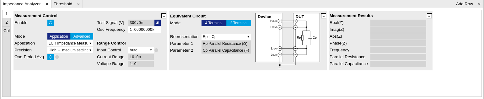
The Impedance Analyzer tab shown in Figure 2 is open by default and provides you with the necessary settings to start measuring impedance. For a quick measurement of the 1 kΩ device-under-test (DUT), the default settings are suitable. All we have to do is to click the Enable button on top left of the Impedance Analyzer tab in order to turn on the drive signal and start the measurement. Since automatic range control is enabled by default, the current and voltage input ranges will be adjusted within a few seconds and the measurement starts.

Figure 2: Impedance Analyzer tab (Application mode)

The measurement result is now shown in the Measurement Results section of the tab. As an alternative, the Numeric Tab provides a more configurable display of the data. Open the tab by clicking on the corresponding icon on the left of the screen. The Numeric tab shown in Figure 3 is organized in panels which display the impedance Z_DUT in Cartesian and in polar form and other parameters. You can add more panels using the Tree Selector on the right if you wish to monitor other quantities such as bias voltage. Every numerical value is supported by a graphical bar scale indicator for better readability. We read an impedance absolute value Abs(Z) of 999.8 Ω, and a complex phase Phase(Z) of nearly 0 degrees, nicely corresponding to the 1 kΩ DUT that we plugged in.

Figure 3: Numerical tab displaying measured impedance and circuit representation parameters

Measure Frequency Dependence¶

The frequency is a critical measurement parameter. The frequency can be changed manually by clicking on the Osc Frequency field, typing a value such as 1000 or 1k in short press either Tab or Enter on your keyboard to apply the setting. For a more systematic measurement of the frequency dependence, we’ll turn to the Sweeper tool .

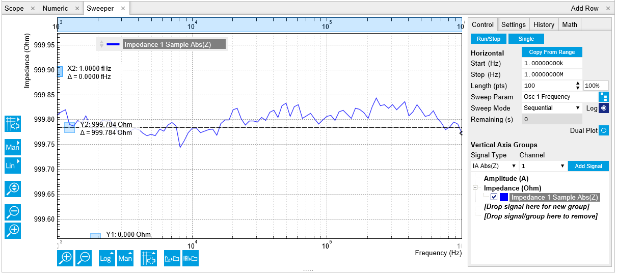
Open the Sweeper tab by clicking on the corresponding icon on the left side of the user interface. The Sweeper features an Application Mode providing suitable settings for common applications. An Advanced mode gives access to detailed settings in order to fully customize averaging and precision, bandwidth, sweeper speed, and so forth. By default, the Sweeper plot area contains the absolute value of the impedance, as well as the Representation Parameters 1 and 2. In the Control sub-tab you can configure the sweep parameter, the sweep range and resolution. Set the start and stop frequency to 1 kHz and 1 MHz. By default, the sweeper is set to divide this span into 100 points on a logarithmic grid. Both of these settings are configurable, as well as the Sweep Parameter. The following table summarizes the Sweeper settings we use.

Table 1: Settings: configure the Sweeper for frequency dependence measurement
Tab	Sub-tab	Section	Label	Setting / Value / State
Sweeper	Settings		Filter	Application Mode
Sweeper	Settings		Application	Impedance
Sweeper	Control	Horizontal	Sweep Param	Osc 1 Frequency
Sweeper	Control	Horizontal	Start / Stop	1k / 1M
Sweeper	Control	Horizontal	Length	100 pts

Start the frequency sweep by clicking on . The screenshot in Figure 4 shows the measurement in the plot section of the Sweeper tab. It shows a perfectly flat curve for the real part of the impedance Abs(Z) within 0.05% of 1 kΩ as is indicated with the cursor for the vertical axis. Whereas our 1 kΩ DUT has no notable frequency dependence between 1 Hz and 1 MHz, very large or small resistors will typically show a change in Abs(Z) towards high frequencies due to the spurious capacitance or inductance.

The plot section features multi-trace and dual-plot functionalities for representing multiple curves with different units, such as Ohm (Ω) and Farad (F), or with very different magnitudes. The plot functionality in LabOne is described in more detail in Plot Functionality. There you also find a description of the cursor and math functions for quick quantitative analysis of measurement data.

Figure 4: LabOne Sweeper showing the frequency dependence of a 1 kΩ DUT

Circuit Representation and Measurement Mode¶

There are two settings that any user should be aware of before continuing with own measurements: the Equivalent Circuit Mode, and the DUT Representation. These settings determine the currently active measurement configuration. The configuration is graphically represented by a dynamically updated circuit diagram in the Impedance Analyzer tab.

The Measurement Mode (either 2 Terminal or 4 Terminal) corresponds to the way the DUT is wired to the instrument connectors. This determines where the DUT voltage V is measured: on L_POT and H_POT, or on H_CUR. The voltage measurement together with the measurement of the current I on L_POT constitutes a measurement of the impedance Z=V/I. For the 1 kΩ DUT, the measurement mode is 4 Terminal because all four connectors H_CUR, L_POT, H_POT and L_POT are wired to the DUT.
The DUT Representation determines how the measured complex-valued impedance Z_DUT=V/I is converted into DUT circuit parameters such as resistance and capacitance. For our 1 kΩ resistor, a parallel resistor-capacitor representation Rp || Cp makes sense, even if the parallel capacitance is negligible.

More general information about the DUT model and the measurement mode is found in Impedance and its Measurement . The DUT representation parameters (in our case Representation Parameter 1 = Rp, and Representation Parameter 2 = Cp) are available for display elsewhere in the user interface, e.g. in the Numeric or in the Sweeper tab. In the Numeric tab shown in Figure 3, the Model Parameter 1 (Rp) reads 999.8 Ω. The panel of the Model Parameter 2 (Cp) shows no numerical reading but the message "Suppression" instead. This message of the LabOne Confidence Indicator informs you in situations when one of the Model Parameters cannot be determined reliably. In the present case, the current passing through the stray capacitance between the resistor electrodes is too small compared to the current through the resistor itself. Instead of displaying a calculated numeric value with no meaning, the "Suppression" warning prevents you from doing systematic measurement errors.

Apart from "Suppression", there are other Confidence Indicator warnings that can appear. The Confidence Indicator is for instance able to detect missing connections (e.g. when tying to measure a DUT in 4 Terminal mode when it is connected to 2 terminals only), or signal underflow and overflow conditions. The meanings of the different warnings are summarized in List of warning messages provided by the Confidence Indicator. in the Functional Description chapter.

Time Dependence and Filtering¶

Next, we will have a look at the Plotter tab that allows users to observe measurement data as a function of time, e.g. to measure the long-term stability of a component impedance. Open the Plotter tab by clicking on the corresponding icon on the left, and choose the Impedance preset in the Control sub-tab in order to add a selection of useful quantities to the plot. It is possible to adjust the scaling of the graph in both directions, or make detailed measurements with 2 cursors for each direction. Try zooming in along the time dimension using the mouse wheel or the icons below the graph. When zooming in far enough, the mode in which the data are displayed will change from a min-max envelope plot to linear point interpolation depending on the density of points along the horizontal axis as compared to the number of pixels available on the screen. For a good overview, disable all traces except the resistance (Impedance 1 Representation Parameter 1) using the checkboxes in the Vertical Axis Group section.

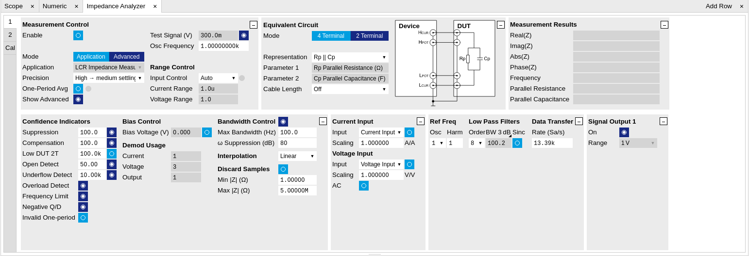
The Plotter is a good tool to observe the noise in the measurement. Noise can be efficiently eliminated by low-pass filtering. The MFIA offers automatic bandwidth control which usually provides good noise reduction without unnecessarily slowing down the measurement. Nonetheless it can sometimes be beneficial to optimize the filtering manually, for instance in situations with strong electrical noise. For manual adjustment, disable the Bandwidth Control button in the Impedance Analyzer tab. This setting is only visible in the lower half of the IA tab after setting Mode to Advanced in the Measurement Control section, see Figure 5. The Low-Pass Filters section now changes from a disabled (greyed-out) state to an editable (white) state. Try different filter bandwidths, e.g. 1 Hz and 100 Hz, to see the live effect on the data as seen in Figure 6. More information about filter parameters is found in the Signal Processing Basics.

Figure 5: Impedance Analyzer tab (Advanced mode)

Figure 6: LabOne Plotter showing a resistance measurement over time. Changing the filter setting manually leads to a change in noise.

The following table summarizes the Plotter settings we use.

Table 2: Settings: configure the Sweeper for frequency dependence measurement
Tab	Sub-tab	Section	Label	Setting / Value / State
Plotter	Control	Select a Preset		Impedance
IA		Measurement Control	Mode	Advanced
IA		Bandwidth Control	Auto	OFF
IA		Low-Pass Filters	BW 3dB	1 Hz / 100 Hz

Measurement Accuracy¶

The measurement accuracy is one of the key specifications of an impedance analyzer. It relates the measured and the real DUT impedance , see Impedance and its Measurement . The real impedance of the supplied 1 kΩ DUT is within 0.05% of an ideal 1 kΩ resistor in the frequency range of the MFIA, and is therefore suitable to judge the accuracy of the measurement result.

The measurement accuracy is not a universal number but depends on the frequency and on the absolute impedance |Z_DUT|. Figure 7 shows the accuracy across the full parameter space covered by the MFIA. This impedance accuracy chart is a handy tool not only to get the measurement accuracy, but also to quickly obtain the absolute impedance of a capacitance or inductance at a certain frequency. For 1 kΩ (vertical axis) and 1 kHz (horizontal axis), we land in a region with 0.05% accuracy.

Figure 7: Impedance Accuracy chart

Note

The relative accuracy specification of the instrument applies to the measured total impedance. Neither does it apply to the real or imaginary parts of the impedance individually, nor to the circuit representation parameters. A 30 minute warm-up time and a 300 mV test signal are required to reach the maximum accuracy.