User Interface Overview
UI Nomenclature
This section provides an overview of the LabOne User Interface, its main elements and naming conventions. The LabOne User Interface is a browser-based UI provided as the primary interface to the MFIA instrument. Multiple browser sessions can access the instrument simultaneously and the user can have displays on multiple computer screens. Parallel to the UI, the instrument can be controlled and read out by custom programs written in any of the supported languages (e.g. LabVIEW, MATLAB, Python, C) connecting through the LabOne APIs.

The LabOne User Interface automatically opens some tabs by default after a new UI session has been started. At start-up, the UI is divided into two tab rows, each containing a tab structure that gives access to the different LabOne tools. Depending on display size and application, tab rows can be freely added and deleted with the control elements on the right-hand side of each tab bar. Similarly, the individual tabs can be deleted or added by selecting app icons from the side bar on the left. A click on an icon adds the corresponding tab to the display, alternatively the icon can be dragged and dropped into one of the tab rows. Moreover, tabs can be moved by drag-and-drop within a row or across rows.
Table 1 gives a brief descriptions and naming conventions for the most important UI items.
| Item name | Position | Description | Contains |
|---|---|---|---|
| side bar | left-hand side of the UI | contains app icons for each of the available tabs - a click on an icon adds or activates the corresponding tab in the active tab row | app icons |
| status bar | bottom of the UI | contains important status and warning indicators, device and session information, and access to the command log | status indicators |
| main area | center of the UI | accommodates all active tabs – new rows can be added and removed by using the control elements in the top right corner of each tab row | tab rows, each consisting of tab bar and the active tab area |
| tab area | inside of each tab | provides the active part of each tab consisting of settings, controls and measurement tools | sections, plots, sub-tabs, unit selections |
Further items are highlighted in Figure 2.

Unique Set of Analysis Tools
All instruments feature a comprehensive tool set for time and frequency domain analysis for both raw and demodulated signals.
The app icons on the left side of the UI can be roughly divided into two categories: settings and tools.
Settings-related tabs are in direct connection to the instrument hardware, allowing the user to control all the settings and instrument states.
Tools-related tabs place a focus on the display and analysis of gathered measurement data.
There is no strict distinction between settings and tools, e.g. the Sweeper will change certain demodulator settings while performing a frequency sweep. Within the tools one can often further discriminate between time domain and frequency domain analysis. Moreover, a distinction can be made between the analysis of fast input signals - typical sampling rate of 60 MSa/s - and the measurement of orders of magnitude slower data - typical sampling rate of <200 kSa/s - derived for instance from demodulator outputs and auxiliary inputs. Table 2 provides a brief classification of the tools.
| Time Domain | Frequency Domain | |
|---|---|---|
| Fast signals (60 MSa/s) | Oscilloscope (Scope tab) | FFT Analyzer (Scope tab) |
| Slow signals (<200 kSa/s) | Numeric | Spectrum Analyzer (Spectrum tab) |
| Plotter | Sweeper | |
| Data Acquisition | - |
The following table gives the overview of all app icons. Note that the selection of app icons may depend on the upgrade options installed on a given instrument.
| Control/Tool | Option/Range | Description |
|---|---|---|
| IA | Quick overview and access to all the settings and properties for impedance measurements. | |
| Files | Access files on internal flash memory and USB drive. | |
| Numeric | Access to all continuously streamed measurement data as numerical values. | |
| Plotter | Displays various continuously streamed measurement data as traces over time (roll mode). | |
| Scope | Displays shots of data samples in time and frequency domain (FFT) representation. | |
| DAQ | Provides complex trigger functionality on all continuously streamed data samples and time domain display. | |
| Spectrum | Provides FFT functionality to all continuously streamed measurement data. | |
| Sweeper | Sweep frequencies, voltages, and other quantities over a defined range and display various response functions including statistical operations. | |
| Lock-in | Quick overview and access to all the settings and properties for signal generation and demodulation. | |
| Lock-in MD | Quick overview and access to all the settings and properties for signal generation and demodulation. | |
| Aux | Controls all settings regarding the auxiliary inputs and auxiliary outputs. | |
| In/Out | Gives access to all controls relevant for the Signal Inputs and Signal Outputs of each channel. | |
| DIO | Gives access to all controls relevant for the digital inputs and outputs including DIO, Trigger Inputs, Trigger Outputs, and Marker Outputs. | |
| Config | Provides access to software configuration. | |
| Device | Provides instrument specific settings. | |
| PID | Features all control, analysis, and simulation capabilities of the PID controllers. | |
| MOD | Control panel to enable (de)modulation at linear combinations of oscillator frequencies. | |
| Boxcar | Boxcar settings for fast input signals. | |
| MDS | Synchronize multiple instruments. | |
| ZI Labs | Experimental settings and controls. |
Table 4 provides a quick overview over the different status bar elements along with a short description.
| Control/Tool | Option/Range | Description |
|---|---|---|
| Command log | last command | Shows the last command. A different formatting (MATLAB, Python, ..) can be set in the config tab. The log is also saved in [User]\Documents\Zurich Instruments\LabOne\WebServer\Log |
| Show Log |  |
Show the command log history in a separate browser window. |
| Errors | Errors | Display system errors in separate browser tab. |
| Device | devXXX | Indicates the device serial number. |
| Identify Device |  |
When active, device LED blinks |
| Shutdown | Shuts down the instrument. | |
| MDS | grey/green/red/yellow | Multiple device synchronization indicator. Grey: Nothing to synchronize - single device on the UI. Green: All devices on the UI are correctly synchronized. Yellow: MDS sync in progress or only a subset of the connected devices is synchronized. Red: Devices not synchronized or error during MDS sync. |
| REC | grey/red | A blinking red indicator shows ongoing data recording (related to global recording settings in the Config tab). |
| IA | grey/green | Impedance Analyzer - Green: indicates which of the impedance analyzer modules is enabled. |
| CF | grey/yellow/red | Clock Failure - Red: present malfunction of the external 10 MHz reference oscillator. Yellow: indicates a malfunction occurred in the past. |
| OVI | grey/yellow/red | Signal Input Overload - Red: present overload condition on the signal input also shown by the red front panel LED. Yellow: indicates an overload occurred in the past. |
| OVO | grey/yellow/red | Overload Signal Output - Red: present overload condition on the signal output. Yellow: indicates an overload occurred in the past. |
| COM | grey/yellow/red | Packet Loss - Red: present loss of data between the device and the host PC. Yellow: indicates a loss occurred in the past. |
| COM | grey/yellow/red | Sample Loss - Red: present loss of sample data between the device and the host PC. Yellow: indicates a loss occurred in the past. |
| COM | grey/red | Stall - Red: indicates that the sample transfer rates have been reset to default values to prevent severe communication failure. This is typically caused by high sample transfer rates on a slow host computer. |
| Reset status flags | Clear the current state of the status flags | |
| MOD | grey/green | MOD - Green: indicates which of the modulation kits is enabled. |
| PID | grey/green | PID - Green: indicates which of the PID units is enabled. Red: indicates PID unit is in PLL or ExtRef mode but is not locked. Yellow: indicates PID unit was not locked in the past. |
| PLL | grey/green | PLL - Green: indicates which of the PLLs is enabled. |
| Full Screen |  |
Toggles the browser between full screen and normal mode. |
Plot Functionality
Several tools provide a graphical display of measurement data in the form of plots. These are multi-functional tools with zooming, panning and cursor capability. This section introduces some of the highlights.
Plot Area Elements
Plots consist of the plot area, the X range and the range controls. The X range (above the plot area) indicates which section of the wave is displayed by means of the blue zoom region indicators. The two ranges show the full scale of the plot which does not change when the plot area displays a zoomed view. The two axes of the plot area instead do change when zoom is applied.
The mouse functionality inside of a plot greatly simplifies and speeds up data viewing and navigation.
| Name | Action | Description | Performed inside |
|---|---|---|---|
| Panning | left click on any location and move around | moves the waveforms | plot area |
| Zoom X axis | mouse wheel | zooms in and out the X axis | plot area |
| Zoom Y axis | shift + mouse wheel | zooms in and out the Y axis | plot area |
| Window zoom | shift and left mouse area select | selects the area of the waveform to be zoomed in | plot area |
| Absolute jump of zoom area | left mouse click | moves the blue zoom range indicators | X and Y range, but outside of the blue zoom range indicators |
| Absolute move of zoom area | left mouse drag-and-drop | moves the blue zoom range indicators | X and Y range, inside of the blue range indicators |
| Full Scale | double click | set X and Y axis to full scale | plot area |
Each plot area contains a legend that lists all the shown signals in the respective color. The legend can be moved to any desired position by means of drag-and-drop.
The X range and Y range plot controls are described in Table 6.
Note
Plot data can be conveniently exported to other applications such as Excel or Matlab by using LabOne’s Net Link functionality, see LabOne Net Link for more information.
| Control/Tool | Option/Range | Description |
|---|---|---|
| Axis scaling mode |  |
Selects between automatic, full scale and manual axis scaling. |
| Axis mapping mode |  |
Select between linear, logarithmic and decibel axis mapping. |
| Axis zoom in | Zooms the respective axis in by a factor of 2. | |
| Axis zoom out | Zooms the respective axis out by a factor of 2. | |
| Rescale axis to data | Rescale the foreground Y axis in the selected zoom area. | |
| Save figure | Generates PNG, JPG or SVG of the plot area or areas for dual plots to the local download folder. | |
| Save data | Generates a CSV file consisting of the displayed wave or histogram data (when histogram math operation is enabled). Select full scale to save the complete wave. The save data function only saves one shot at a time (the last displayed wave). | |
| Cursor control |  |
Cursors can be switch On/Off and set to be moved both independently or one bound to the other one. |
| Net Link | Provides a LabOne Net Link to use displayed wave data in tools like Excel, MATLAB, etc. |
Cursors and Math
The plot area provides two X and two Y cursors which appear as dashed lines inside of the plot area. The four cursors are selected and moved by means of the blue handles individually by means of drag-and-drop. For each axis, there is a primary cursor indicating its absolute position and a secondary cursor indicating both absolute and relative position to the primary cursor.
Cursors have an absolute position which does not change upon pan or zoom events. In case a cursor position moves out of the plot area, the corresponding handle is displayed at the edge of the plot area. Unless the handle is moved, the cursor keeps the current position. This functionality is very effective to measure large deltas with high precision (as the absolute position of the other cursors does not move).
The cursor data can also be used to define the input data for the mathematical operations performed on plotted data. This functionality is available in the Math sub-tab of each tool. The Table 7 gives an overview of all the elements and their functionality. The chosen Signals and Operations are applied to the currently active trace only.
Note
Cursor data can be conveniently exported to other applications such as Excel or MATLAB by using LabOne’s Net Link functionality, see LabOne Net Link for more information.
| Control/Tool | Option/Range | Description |
|---|---|---|
| Source Select | Select from a list of input sources for math operations. | |
| Cursor Loc | Cursor coordinates as input data. | |
| Cursor Area | Consider all data of the active trace inside the rectangle defined by the cursor positions as input for statistical functions (Min, Max, Avg, Std). | |
| Tracking | Display the value of the active trace at the position of the horizontal axis cursor X1 or X2. | |
| Plot Area | Consider all data of the active trace currently displayed in the plot as input for statistical functions (Min, Max, Avg, Std). | |
| Peak | Find positions and levels of up to 5 highest peaks in the data. | |
| Trough | Find positions and levels of up to 5 lowest troughs in the data. | |
| Histogram | Display a histogram of the active trace data within the x-axis range. The histogram is used as input to statistical functions (Avg, Std). Because of binning, the statistical functions typically yield different results than those under the selection Plot Area. | |
| Resonance | Display a curve fitted to a resonance. | |
| Linear Fit | Display a linear regression curve. | |
| Operation Select | Select from a list of mathematical operations to be performed on the selected source. Choice offered depends on the selected source. | |
| Cursor Loc: X1, X2, X2-X1, Y1, Y2, Y2-Y1, Y2 / Y1 | Cursors positions, their difference and ratio. | |
| Cursor Area: Min, Max, Avg, Std | Minimum, maximum value, average, and bias-corrected sample standard deviation for all samples between cursor X1 and X2. All values are shown in the plot as well. | |
| Tracking: Y(X1), Y(X2), ratioY, deltaY | Trace value at cursor positions X1 and X2, the ratio between these two Y values and their difference. | |
| Plot Area: Min, Max, Pk Pk, Avg, Std | Minimum, maximum value, difference between min and max, average, and bias-corrected sample standard deviation for all samples in the x axis range. | |
| Peak: Pos, Level | Position and level of the peak, starting with the highest one. The values are also shown in the plot to identify the peak. | |
| Histogram: Avg, Std, Bin Size, (Plotter tab only: SNR, Norm Fit, Rice Fit) | A histogram is generated from all samples within the x-axis range. The bin size is given by the resolution of the screen: 1 pixel = 1 bin. From this histogram, the average and bias-corrected sample standard deviation is calculated, essentially assuming all data points in a bin lie in the center of their respective bin. When used in the plotter tab with demodulator or boxcar signals, there additionally are the options of SNR estimation and fitting statistical distributions to the histogram (normal and rice distribution). | |
| Resonance: Q, BW, Center, Amp, Phase, Fit Error | A curve is fitted to a resonator. The fit boundaries are determined by the two cursors X1 and X2. Depending on the type of trace (Demod R or Demod Phase) either a Lorentzian or an inverse tangent function is fitted to the trace. The Q is the quality factor of the fitted curve. BW is the 3dB bandwidth (FWHM) of the fitted curve. Center is the center frequency. Amp gives the amplitude (Demod R only), whereas Phase returns the phase at the center frequency of the resonance (demod Phase only). The fit error is given by the normalized root-mean-square deviation. It is normalized by the range of the measured data. | |
| Linear Fit: Intercept, Slope, R² | A simple linear least squares regression is performed using a QR decomposition routine. The fit boundaries are determined by the two cursors X1 and X2. The parameter outputs are the Y-axis intercept, slope and the R²-value, which is the coefficient of determination to determine the goodness-of-fit. | |
| Add |  |
Add the selected math function to the result table below. |
| Add All |  |
Add all operations for the selected signal to the result table below. |
| Clear Selected | Clear selected lines from the result table above. | |
| Clear All | Clear all lines from the result table above. | |
| Copy |  |
Copy selected row(s) to Clipboard as CSV |
| Unit Prefix | Adds a suitable prefix to the SI units to allow for better readability and increase of significant digits displayed. | |
| CSV |  |
Values of the current result table are saved as a text file into the download folder. |
| Net Link |  |
Provides a LabOne Net Link to use the data in tools like Excel, MATLAB, etc. |
| Help |  |
Opens the LabOne User Interface help. |
Note
The standard deviation is calculated using the formula \(\sqrt \frac{1}{N-1}\sum_{i=1}^{N}(x_i-\bar{x})^2\) for the unbiased estimator of the sample standard deviation with a total of N samples \(x_i\) and an arithmetic average \(\bar{x}\). The formula above is used as-is to calculate the standard deviation for the Histogram Plot Math tool. For large number of points (Cursor Area and Plot Area tools), the more accurate pairwise algorithm is used (Chan et al., "Algorithms for Computing the Sample Variance: Analysis and Recommendations", The American Statistician 37 (1983), 242-247).
The fitting functions used in the Resonance Plot Math tool depend on the selected signal source. The demodulator R signal is fitted with the following function:
where \(C\) accounts for a possible offset in the output, \(A\) is the amplitude, \(Q\) is the quality factor and \(f_0\) is the center frequency. The demodulator \(\phi\) signal s fitted with the following function:
using the same parameters as above.
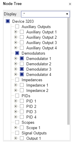
Tree Selector
The Tree selector allows one to access streamed measurement data in a
hierarchical structure by checking the boxes of the signals that should
be displayed. The tree selector also supports data selection from
multiple instruments, where available. Depending on the tool, the Tree
selector is either displayed in a separate Tree sub-tab, or it is
accessible by a click on the  button.
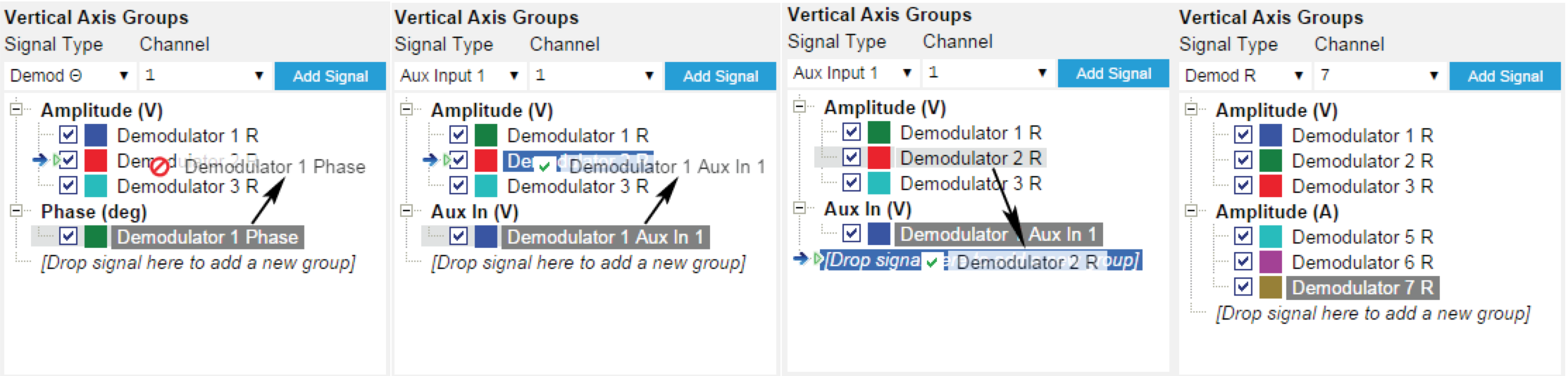
Vertical Axis Groups
Vertical Axis groups are available as part of the plot functionality in many of the LabOne tools. Their purpose is to handle signals with different axis properties within the same plot. Signals with different units naturally have independent vertical scales even if they are displayed in the same plot. However, signals with the same unit should preferably share one scaling to enable quantitative comparison. To this end, the signals are assigned to specific axis group. Each axis group has its own axis system. This default behavior can be changed by moving one or more signals into a new group.

The tick labels of only one axis group can be shown at once. This is the foreground axis group. To define the foreground group click on one of the group names in the Vertical Axis Groups box. The current foreground group gets a high contrast color.
Select foreground group Click on a signal name or group name inside the Vertical Axis Groups. If a group is empty the selection is not performed.
Split the default vertical axis group Use drag-and-drop to move one signal on the field [Drop signal here to add a new group]. This signal will now have its own axis system.
Change vertical axis group of a signal Use drag-and-drop to move a signal from one group into another group that has the same unit.
Group separation In case a group hosts multiple signals and the unit of some of these signals changes, the group will be split in several groups according to the different new units.
Remove a signal from the group In order to remove a signal from a group drag-and-drop the signal to a place outside of the Vertical Axis Groups box.
Remove a vertical axis group A group is removed as soon as the last signal of a custom group is removed. Default groups will remain active until they are explicitly removed by drag-and-drop. If a new signal is added that match the group properties it will be added again to this default group. This ensures that settings of default groups are not lost, unless explicitly removed.
Rename a vertical axis group New groups get a default name "Group of ...". This name can be changed by double-clicking on the group name.
Hide/show a signal Uncheck/check the check box of the signal. This is faster than fetching a signal from a tree again.
| Control/Tool | Option/Range | Description |
|---|---|---|
| Vertical Axis Group | Manages signal groups sharing a common vertical axis. Show or hide signals by changing the check box state. Split a group by dropping signals to the field [Drop signal here to add new group]. Remove signals by dragging them on a free area. Rename group names by editing the group label. Axis tick labels of the selected group are shown in the plot. Cursor elements of the active wave (selected) are added in the cursor math tab. |
|
| Signal Type | HW Trigger | Select signal types for the Vertical Axis Group. |
| Demod X, Y, R, Theta | ||
| Frequency | ||
| Aux Input 1, 2 | ||
| Channel | integer value | Selects a channel to be added. |
| Signal | integer value | Selects signal to be added. |
| Add Signal |  |
Adds a signal to the plot. The signal will be added to its default group. It may be moved by drag and drop to its own group. All signals within a group share a common y-axis. Select a group to bring its axis to the foreground and display its labels. |
| Window Length | 2 s to 12 h | Window memory depth. Values larger than 10 s may cause excessive memory consumption for signals with high sampling rates. Auto scale or pan causes a refresh of the display for which only data within the defined window length are considered. |
Trends
The Trends tool lets the user monitor the temporal evolution of signal features such as minimum and maximum values, or mean and standard deviation. This feature is available for the Scope , Spectrum, Plotter, and DAQ tab. Using the Trends feature, one can monitor all the parameters obtained in the Math sub-tab of the corresponding tab.
The Trends tool allows the user to analyze recorded data on a different and adjustable time scale much longer than the fast acquisition of measured signals. It saves time by avoiding post-processing of recorded signals and it facilitates fine-tuning of experimental parameters as it extracts and shows the measurement outcome in real time.
To activate the Trends plot, enable the Trends button in the Control sub-tab of the corresponding main tab. Various signal features can be added to the plot from the Trends sub-tab in the Vertical Axis Groups . The vertical axis group of Trends has its own Run/Stop button and Length setting independent from the main plot of the tab. Since the Math quantities are derived from the raw signals in the main plot, the Trends plot is only shown together with the main plot. The Trends feature is only available in the LabOne user interface and not at the API level.
