Advanced Impedance Measurements
Note
This tutorial is applicable to all MFIA Instruments and to MFLI Instruments with the MF-IA Impedance Analyzer option installed.
Goals and Requirements
The goal of this tutorial is to show some more advanced features of the LabOne user interface by guiding you through a measurement of a frequency-dependent impedance. We introduce important practical aspects about impedance measurements such as the influence of parasitics, or the effect of parameter suppression.
This tutorial is for people with some starting experience with Zurich Instruments impedance analyzers. To follow this tutorial, you need a 1 MΩ DUT fitting the MFITF Impedance Test Fixture. An easy way to get that is to solder a 1 MΩ through-hole resistor onto one of the DUT carriers delivered with the MFITF.
Preparation
Start by connecting the MFITF Test Fixture to the BNC connectors on the front panel of the MFIA, and plug the DUT into the 8-pin connector on the front of the test fixture. Figure 1 shows a diagram of the hardware setup.

Make sure that the MFIA Instrument is powered on and then connect the MFIA directly by USB to your host computer or by Ethernet to your local area network (LAN) where the host computer resides. After connecting to your Instrument through the web browser using its address or through the MF Device Finder, the LabOne graphical user interface is opened. Check the Getting Started for detailed instructions. The tutorial can be started with the default instrument configuration (e.g. after a power cycle) and the default user interface settings (i.e. as is after pressing F5 in the browser).
Impedance and Representation Parameters
The real impedance of a DUT like the 1 MΩ resistor is not necessarily equal to its nominal, or ideal, value. First of all, the DUT impedance value is only specified within some accuracy, e.g. 1%. In addition to that imperfection, there are spurious impedance components such as lead inductance, or parallel capacitance. For the given 1 MΩ resistor, the real impedance is indeed close to that of a parallel Rp||Cp circuit, with a parallel capacitor Cp of some hundreds of fF. This real impedance, including device imperfections, is what the MFIA measures.
In order to measure the 1 MΩ DUT, we configure the Impedance Analyzer with a suitable Equivalent Circuit Representation of Rp||Cp. Since the DUT carrier we use is connected to 2 leads only, we change the measurement mode to 2 Terminal. Furthermore, we set the Range Control to Auto. This will set the input current and voltage ranges to suitable values.
Table 1 summarizes the instrument settings we use.
| Tab | Sub-tab | Section | # | Label | Setting / Value / State |
|---|---|---|---|---|---|
| IA | Equivalent Circuit | Mode | 2 Terminal | ||
| IA | Equivalent Circuit | Representation | Rp || Cp | ||
| IA | Measurement Control | Osc Frequency | 1 k | ||
| IA | Measurement Control | Enable | ON | ||
| IA | Range Control | Input Control | Auto |
Measure the Frequency Dependence
Open the Sweeper tab (Settings sub-tab), select the Application Mode, and Impedance as the Application. In the Control sub-tab you can configure the sweep parameter, the sweep range and resolution. We choose parameters for a logarithmic frequency sweep from 1 kHz to 1 MHz. We start with a measurement of the absolute impedance |ZDUT|. Add this parameter to the plot by selecting "IA Abs(Z)" as a Signal Type, and click on "Add Signal". The following table summarizes the Sweeper settings we use.
| Tab | Sub-tab | Section | # | Label | Setting / Value / State |
|---|---|---|---|---|---|
| Sweeper | Settings | Filter | Application Mode | ||
| Sweeper | Settings | Application | Impedance | ||
| Sweeper | Control | Horizontal | Sweep Param | Osc 1 Frequency | |
| Sweeper | Control | Horizontal | Start / Stop | 1k / 1M | |
| Sweeper | Control | Horizontal | Length | 100 pts |
Start the frequency sweep by clicking on  .
Display the absolute impedance |ZDUT| by selecting
"Impedance 1 Sample Abs(Z)" in the Vertical Axis Groups section. Naively
we might expect this parameter to stay constant at 1 MΩ, but in fact it
drops by about 50% at 500 kHz. The plot in Figure 2
shows the measurement of |ZDUT| as the red curve in the
plot section of the Sweeper tab. The drop of the absolute impedance is
due to the spurious parallel capacitance. At high enough frequencies,
this capacitance forms a bypass for the current and therefore leads to a
reduction of the impedance.
.
Display the absolute impedance |ZDUT| by selecting
"Impedance 1 Sample Abs(Z)" in the Vertical Axis Groups section. Naively
we might expect this parameter to stay constant at 1 MΩ, but in fact it
drops by about 50% at 500 kHz. The plot in Figure 2
shows the measurement of |ZDUT| as the red curve in the
plot section of the Sweeper tab. The drop of the absolute impedance is
due to the spurious parallel capacitance. At high enough frequencies,
this capacitance forms a bypass for the current and therefore leads to a
reduction of the impedance.


The Rp || Cp circuit representation allows us to extract the parallel resistance Rp and capacitance Cp separately. Even after the Sweep has finished, we can add these signals to the plot by selecting IA Parameter 1 or IA Parameter 2 as Signal Type, and clicking on "Add Signal". Selecting the corresponding Impedance 1 Sample Rep Parameter 1 or 2 in the Vertical Axis Groups section will change the axis between a Farad (F) and an Ohm (Ω) scale.
Ideally, the resistance and capacitance are both frequency-independent. Looking at the blue curve in Figure 2 (Rp) and the green curve in Figure 3 (Cp), this is indeed mostly the case in the measurement: Rp stays flat at about 1 MΩ up to a few 100 kHz, and Cp stays at about 0.5 pF. However, parts of both curves are tagged by the Confidence Indicator warning "Suppression". It shows that the capacitance measurement is most reliable at high frequencies, and the resistance measurement is most reliable at low frequencies.
Measure a Nyquist Plot
Instead of a conventional frequency dependence with the frequency on the horizontal axis and an impedance parameter on the vertical axis, the Sweeper also features measurement of Nyquist plots. A Nyquist plot is a parametric plot of the impedance as a function of frequency with the real part of the impedance (resistance) on the horizontal axis, and the imaginary part (reactance) on the vertical axis. To obtain a Nyquist plot, please follow the instructions below.
In the Control sub-tab of the Sweeper, select the desired start
frequency and stop frequency. Set XY Mode to On - Invert and select
Real(Z) as the X signal from the selection tree. Select the imaginary
part of Z with IA Imag(Z) as a Signal Type in the Vertical Axis Groups
and add it to the plot. Start the sweep by clicking on .
Scale the vertical axis by setting the axis scaling mode on the left
side of the plot to Auto, see Plot Area
Elements.
The horizontal axis can be fixed to match the scale of the vertical axis
by using the Track axis scaling mode instead of FS, Manual, or Auto.
This ensures that a circle in the complex plane is displayed as a circle
in the plot independent of the window aspect ratio.
The table below summarizes the settings necessary to obtain a Nyquist plot
| Tab | Sub-tab | Section | # | Label | Setting / Value / State |
|---|---|---|---|---|---|
| Sweeper | Control | XY Mode | On - Invert | ||
| Sweeper | Control | X Signal | Impedances / Impedance 1 Sample / Real(Z) | ||
| Sweeper | Control | Vertical Axis Groups | Signal Type | IA Imag(Z) | |
| Sweeper | Control | Vertical Axis Groups | Add Signal | Click | |
| Sweeper | Plot Area (left) | Axis Scaling Mode | Auto | ||
| Sweeper | Plot Area (bottom) | Axis Scaling Mode | Track |
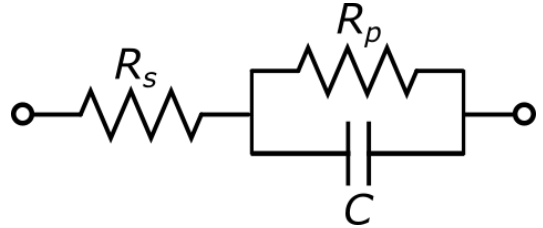
The 1 MΩ resistor connected as a DUT in the setup Figure 1 for this tutorial has relatively unspectacular, linear Nyquist plot. To illustrate the characteristics of a Nyquist plot better, we show the measurement of an R-R-C circuit which has the shape of a semicircle. The measurement shown in Figure 4 is easy to reproduce by soldering the sample from through-hole components as shown in Figure 5 onto a through-hole DUT carrier. The components used here were Rp = 6.8 kΩ, Rs = 2.2 kΩ, and C = 1 µF.

Saving and Exporting Data
Data acquired with the Sweeper can be easily saved to comma-separated value (CSV), MATLAB, and ZView format. Particularly the ZView format is attractive for further equivalent circuit modeling with specialized software tools. Such an analysis often enables precise characterization of the DUT circuit, going much beyond the extraction of a pair of representation parameters.
All past sweeps are listed in the History sub-tab of the Sweeper, up to
a maximum number of list entry specified by the History Length
parameter. Clicking on  will store all the sweeps that are currently in the History list. The
data are stored in a subfolder of the LabOne Data folder which can be
conveniently accessed in the
File Manager Tab.
The Enable button next to each History entry controls the plot display,
but not which sweeps are saved. Find more information, for instance on
how to use the Reference feature, in
Sweeper Tab.
Select your preferred file format from the drop-down list at the bottom
of the History sub-tab of the Sweeper. This setting is global and also
applies to the Plotter and the DAQ tabs.
will store all the sweeps that are currently in the History list. The
data are stored in a subfolder of the LabOne Data folder which can be
conveniently accessed in the
File Manager Tab.
The Enable button next to each History entry controls the plot display,
but not which sweeps are saved. Find more information, for instance on
how to use the Reference feature, in
Sweeper Tab.
Select your preferred file format from the drop-down list at the bottom
of the History sub-tab of the Sweeper. This setting is global and also
applies to the Plotter and the DAQ tabs.
Alternatively, the buttons ![]() and
and ![]() in the plot area of the Sweeper tab allow you to save the selected
graphical traces as a text file or a vector graphics.
in the plot area of the Sweeper tab allow you to save the selected
graphical traces as a text file or a vector graphics.