Compensation
Note
This tutorial is applicable to all MFIA Instruments and to MFLI Instruments with the MF-IA Impedance Analyzer option installed.
Goals and Requirements
The goal of this tutorial is to demonstrate a user compensation for impedance measurements with the MFIA instrument. A compensation improves the measurement accuracy when using a custom impedance fixture.
Some starting experience with Zurich Instruments impedance analyzers is required to follow the tutorial. You also need a Kelvin probe cable set and a 1 Ω through-hole resistor, a 10 Ω resistor, and a simple piece of wire. Instead of the Kelvin probe set, you can use a set of BNC cables and crocodile clamps.
Preparation
Start by connecting the Kelvin probe set to the BNC connectors on the front panel of the MFIA, paying attention not to mix up the connectors. One clamp should be electrically connected to Signal Output +V and Signal Input +V, the other clamp to Signal Input I and Signal Input -V. Fix the 1 Ω resistor with the two clamps. Figure 1 shows a diagram of the hardware setup.

Make sure that the MFIA Instrument is powered on and then connect the MFIA directly by USB to your host computer or by Ethernet to your local area network (LAN) where the host computer resides. After connecting to your Instrument through the web browser using its address, the LabOne graphical user interface is opened. Check the Getting Started for detailed instructions. The tutorial can be started with the default instrument configuration (e.g. after a power cycle) and the default user interface settings (i.e. as is after pressing F5 in the browser).
Configure the Impedance Analyzer
A measurement fixture like the Kelvin probe set affects the impedance measurement through its electrical properties, such as its stray capacitance, or the delay caused by its cables. A carefully executed compensation can practically eliminate the negative influence and thus improve measurement accuracy.
To get an idea of the Kelvin probe’s influence, let’s first make a quick measurement without compensation. We’ll select the Rs+Ls Representation in the Impedance Analyzer tab, which is a good choice for small-valued resistors. The two representation parameters can be read in the Numeric tab with activated Impedance preset. We furthermore relax the threshold of the Suppression warning by setting Suppression Ratio to 100 in the Impedance Analyzer tab. This setting becomes visible in the lower half of the tab after setting the Measurement Control Mode to Advanced. The relaxed condition is deemed sufficient for the level of accuracy that we can achieve with such a cable-based setup.
Let’s start by reading some measurement values at different oscillator frequencies, which we change manually in the Impedance Analyzer tab.
| Frequency | Rep. parameter 1 (resistance Rs) | Rep. parameter 2 (inductance Ls) |
|---|---|---|
| 1 kHz | 1.001 Ω | Suppression |
| 500 kHz | 0.986 Ω | 110 nH |
| 3 MHz | 0.738 Ω | 112 nH |
| 5 MHz (MF-5M option) | Suppression | 111 nH |
The resistance (Rep. parameter 1) at 1 kHz looks quite reasonable. The inductance (Rep. parameter 2) is not reliably measurable at this frequency and is flagged with the "Suppression" warning. At higher frequencies such as 500 kHz, the inductance is measurable, but it seems unexpectedly large: 110 nH would correspond to 10 to 15 cm of wire, but the resistor leads are much shorter. The spurious series inductance Ls of a through-hole component is typically of the order of 5 nH. At 3 MHz the measured resistance drops to 0.738 Ω which does not seem realistic. At the maximum frequency 5 MHz, the resistance measurement finally fails. The following table summarizes the settings we used.
| Tab | Sub-tab | Section | # | Label | Setting / Value / State |
|---|---|---|---|---|---|
| IA | Equivalent Circuit | Representation | Rs + Ls | ||
| IA | Measurement Control | Enable | ON | ||
| IA | Measurement Control | Mode | Advanced | ||
| IA | Confidence Indicators | Suppression | 100 | ||
| IA | Measurement Control | Osc Frequency | 1k, 500k, 3M, 5M |
Carry out the Compensation
Some of the apparent problems seen before can be attributed to the uncompensated Kelvin probe set. In order to do a compensation, open the Cal side-tab in the Impedance Analyzer tab and select the SL (short-load) Compensation Sequence. It’s necessary to specify the parameters of the reference "load" DUT, such as 10 Ω, and since we don’t know precisely its stray capacitance, we’ll enter a value of 0 F as Load C. The compensation steps can now be simply carried out by fixing the appropriate DUT (the wire for the S step, and the 10 Ω resistor for the L step) and clicking on the "Short" or "Load" button followed by "Compensate". For a precise calibration, try to keep the position of the clamps the same in both steps and in the measurement itself. The spurious capacitance is very sensitive to the position of the clamps and the parts of the cables which are unshielded.
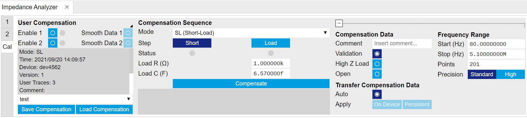
Each compensation step takes about a minute with the standard settings, and its progress and termination is reported in the text field below the "Compensate" button. The Status LEDs show which of the steps are completed. Once all three are done, the compensation data are transferred to the instrument. Compensation files can be saved and reloaded as necessary.
| Tab | Sub-tab | Section | # | Label | Setting / Value / State |
|---|---|---|---|---|---|
| IA | Cal | Compensation Sequence | Mode | SOL (short-load) | |
| IA | Cal | Compensation Sequence | Load R (Ω) | 10 | |
| IA | Cal | Compensation Sequence | Load C (F) | 0 | |
| IA | Cal | Compensation Sequence | Step | Short / Load | |
| IA | Cal | Compensation Sequence | Compensate | ON |
The left section of the Cal side-tab displays information and contains the enable button of the current user compensation and the internal calibration. The label User Compensation (or Internal Calibration) acts as a control to switch the display (the small black triangle to the bottom right of the label indicates the control). When switched to User Compensation, the compensation can easily be activated and deactivated with the Enable button. This has an immediate effect on the measurement data displayed in the Numeric, the Plotter, or the Sweeper tab.
Note
The internal calibration should normally be enabled at all times.
Measure with Compensation
In order to compare the results with and without compensation, we’ll perform a sweep up to the maximum available frequency as shown in the previous tutorials. In the Sweeper tab, perform a linear frequency sweep from 1 kHz to 5 MHz. Repeat that once with and once without enabled compensation.
We look at two selected quantities in the following plots in Figure 3. The Resistance (= Rep. Parameter 1) remains flat at 1.0 Ω with compensation (green), whereas it goes down below 0.4 Ω without compensation.

The Inductance (= Parameter 2) is relatively flat in frequency both with and without compensation, see Figure 4. But its value is much too large without compensation. With compensation the measured value is less than 10 nH which is the expected order of magnitude, in any case it is too small to be measured with high precision and is flagged with the "Suppression" warning. Note that the lead inductance of the resistor is about 8 nH/cm. Clamping the DUT at a slightly different position and measuring again will show an effect on the measured inductance Ls, whereas the resistance Rs is largely insensitive to that.
