Power Spectrum Density Measurement¶

Note

This tutorial is applicable to all SHFQA+ Instruments.

Goals and Requirements¶

The goal of this tutorial is to demonstrate how to use the SHFQA+ to perform power spectral density measurement using the LabOne User Interface (UI) and Zurich Instruments Toolkit API.

Note

For zhinst-toolkit users, please find the example in https://github.com/zhinst/zhinst-toolkit/blob/main/examples/shfqa_shfqc_power_spectral_density.md, and the zhinst-toolkit documentation.

Preparation¶

Please follow the preparation steps in Connecting to the Instrument and connect the instrument in a loopback configuration as shown in Figure 1 or to a device under test.

Figure 1: SHFQA+ connection.

Tutorial¶

In this tutorial, we use 1 SHFQA+ channel to generate a signal under test, and measure the power spectral density of the signal when it is on and off using another channel.

LabOne UIzhinst-toolkit

This section shows how to use LabOne UI to configure the instrument, run the measurement and monitor the measurement results.

Configure the instrument

Set center frequency and power range of input and output signals

Configure these parameters on the Input and Output Tab as in and in Table 1.

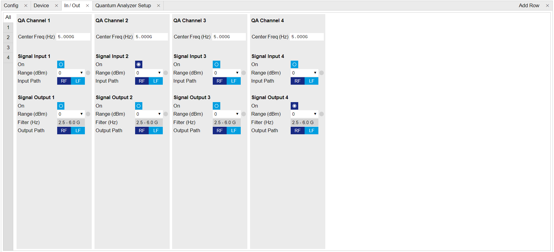
Table 1: Settings on In/Out Tab
Parameter	Setting	Description
QA Channel Selection	All	Select All to display all QA Channels.
Cent Freq (Hz)	5 GHz	Set center frequency of QA Channel 2 and Channel 4 to 5 GHz.
Signal Input 2 On	Enable	Enable the Signal Input 2.
Signal Input 2 Range (dBm)	0 dBm	Set power range of Signal Input 2 to 0 dBm. This setting allows the instrument to acquire a input signal with a power up to 0 dBm.
Signal Input 2 Input Path	RF	Set input path of the Signal Input 2 to RF path.
Signal Output 4 On	Enable	Enable the Signal Output 4.
Signal Output 4 Range	0 dBm	Set power range of Signal Output 4 to 0 dBm. This setting allows the instrument to output a signal with a power up to 0 dBm.
Signal Output 4 Output Path	RF	Set output path of Signal Output 4 to RF path.

Upload and compile measurement sequence

The measurement sequence is defined on the Sequence Sub-Tab of the Readout Pulse Generator Tab, see Figure 3 and Table 2.

The power spectral density of input signal is measured by calculating square of measurement result after integration at different frequencies as \(S_{xx}(f) = \lim_{N\to\infty} \frac{(\Delta t)^2}{T}|\sum_{n = -N}^{n = N} x_ne^{-i2\pi f n\Delta t}|^2\), where \(\Delta t = 1/f_\mathrm{s}\) is the time step, \(f_\mathrm{s}\) is the sampling rate, \(T = (2N+1)\Delta t\) is the integration length in seconds, \(2N+1\) is the integration length in samples, \(x_n\) is the \(n\)-th complex data of the input signal, \(e^{-i2\pi f n\Delta t}\) is the integration weight. By sweeping the frequency of integration weight, the power spectral density of input signal is calculated by the instrument, and it returns the real-valued power spectral density in units of \(\mathrm{Vrms}^2/\mathrm{Hz}\).

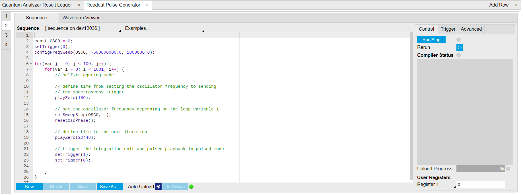
Figure 3: Configurations on Readout Pulse Generator Tab.

Table 2: Settings of QA Channel 2 on Readout Pulse Generator Tab.
Parameter	Setting	Description
QA Channel Selection	2	Select QA channel 2.
Sub-Tab Display	Sequence	Select Sequence sub-tab and paste the sequence program below or load ziGenerator_functional_spectroscopy.seqc from the "Examples" library and modify it.
Compile	Click "To Device"	Compile the sequence program by clicking "To Device".
Return	Disable	Disable return function.
Run/Stop	Disable	Disable Run/Stop.

Below is the the sequence program for the measurement. In the inner loop, the setSweepStep(OSC0, i) command sets frequency of digital oscillator 0 to i-th frequency in an array configured by configFreqSweep(OSC0, -500000000.0, 1000000.0) command, the setTrigger(value) command sets Sequencer Trigger 1 Output to high and then low to start integration, and waveform generation if pulsed waveform is desired, the playZero(samples) command define time to the next playZero(samples). The measurement is repeated 100 times by the outer loop.

// define which oscillator to use
const OSC0 = 0;

// set sequencer trigger output to 0
setTrigger(0);

// configure frequency sweep with a starting f of -500 MHz and a step of 1 MHz
configFreqSweep(OSC0, -500000000.0, 1000000.0);

// sweep oscillator frequency and repeat 100 times
for(var j = 0; j < 100; j++) {
    for(var i = 0; i < 1001; i++) {
        // self-triggering mode

        // define time from setting the oscillator frequency to sending
        // the spectroscopy trigger
        playZero(160);

        // set the oscillator frequency depending on the loop variable i
        setSweepStep(OSC0, i);
        resetOscPhase();

        // define time to the next iteration
        playZero(22448);

        // trigger the integration unit and pulsed playback in pulsed mode
        // set sequencer trigger output 1 to 1 and then to 0
        // make sure the trigger singnal in spectroscopy mode is set to sequencer trigger output 1
        setTrigger(1);
        setTrigger(0);
    }
}

Configure signal generation and data acquisition

The input signal under test is generated using QA Channel 4 as shown in Figure 4 and Table 3.

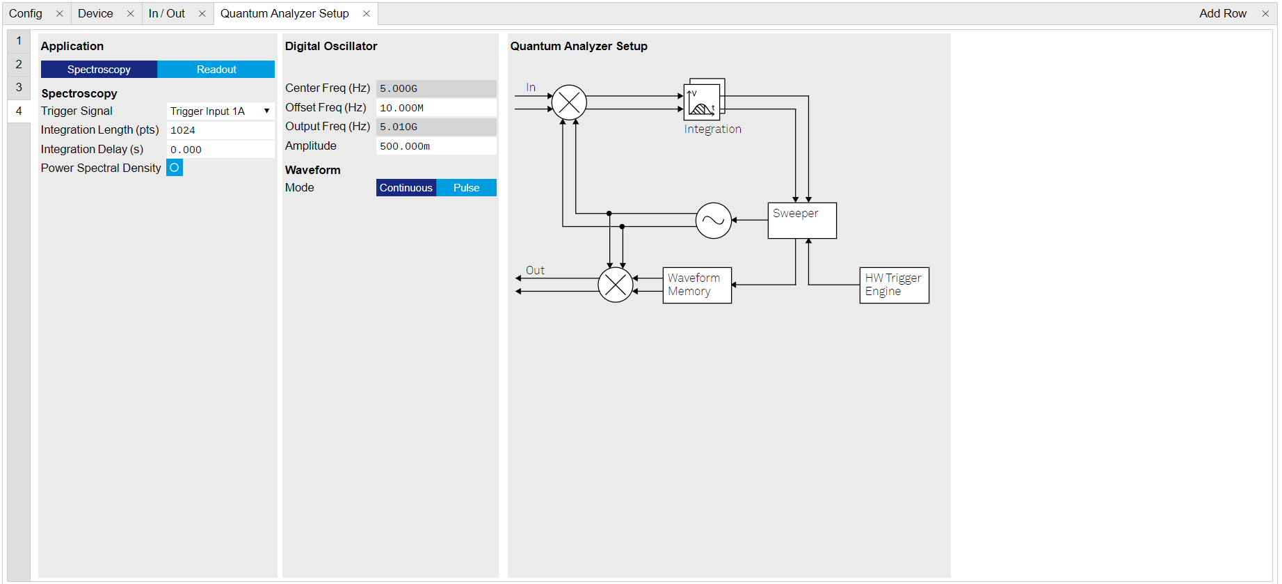
Figure 4: Configurations of QA Channel 4 on QA Setup Tab.

Table 3: Settings of QA Channel 4 on QA Setup Tab.
Parameter	Setting	Description
QA Channel Selection	4	Select QA Channel 4.
Application Mode	Spectroscopy	Use Spectroscopy mode to generate a continuous or pulsed waveform. For simplicity, we generate a continuous wave.
Digital Oscillator Amplitude	0.5	Set the amplitude factor of the digital oscillator to 0.5. The range of amplitude factor is from 0 to 1.
Waveform Mode	Continuous	Set the Waveform Mode to continuous.

Data acquisition are defined on QA Setup Tab and QA Result logger Tab, see Figure 5 and Table 4.

The input signal after frequency down-conversion is integrated at each frequency for 512 ns started 224 ns later after receiving a trigger from Sequencer 1 Trigger Output 1, and the frequency sweep is repeated 100 times. The result after each integration is squared and then averaged cyclically.

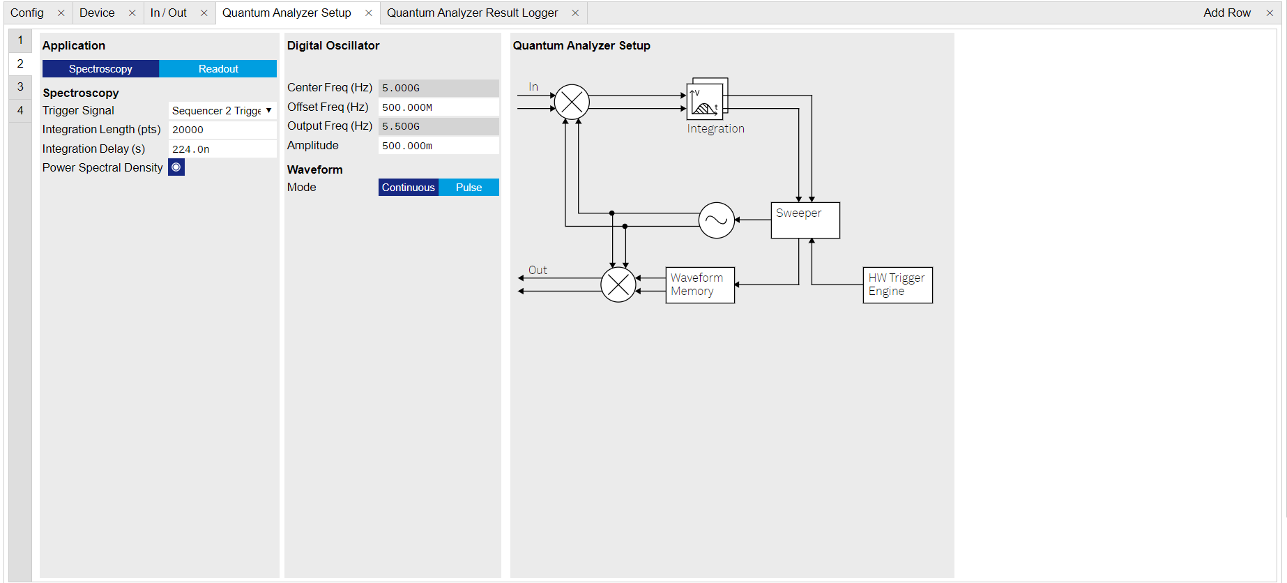
Figure 5: Configurations of QA Channel 2 on QA Setup Tab.

Table 4: Settings of QA Channel 2 on QA Setup Tab.
Parameter	Setting	Description
QA Channel Selection	2	Select QA Channel 2.
Application Mode	Spectroscopy	Use spectroscopy mode for power spectral density measurement.
Trigger Signal	Sequencer 2 Trigger Output 1	Select Sequencer 2 Trigger Output 1 as the trigger source to integration. This selection matches the trigger setting written in the sequence program.
Integration Length (pts)	20000	Set the integration length in number of samples. Note that the integration length which defines measurement bandwidth must to be much longer than \(1/\Delta f\), where \(\Delta f\) is the frequency step set in sequence program. In this tutorial, integration length is 10 \(\mu\)s, and frequency stem is 1 MHz.
Power Spectral Density	Enable	Enable the Power Spectral Density measurement function.

On the QA Result Logger Tab, it defines how the result is averaged and displayed. After all configuration, the QA Result Logger should be enabled to be ready to receive measurement results, see settings in Table 5

Table 5: Settings of QA Channel 2 on QA Result Logger Tab.
Parameter	Setting	Description
QA Channel Selection	2	Select QA Channel 2.
Sub-Tab	Spectroscopy	Select Spectroscopy sub-tab to monitor measurement result when using the Spectroscopy mode.
Plot Type	Components	Select Components to display I, Q, amplitude or phase vs sample points. Select Dot Plot to display I vs Q with scattered dots.
Result Length (Sample)	1001	Set result length in number of samples. The number must match what is set in the sequence program.
Averages	100	Set the number of averages. The number must match what is set in the sequence program.
Average Mode	Cyclic	Set the average mode to cyclic. This setting must match how the loop is configured in the sequence program.
Vertical Axis Groups	Add amplitude and phase	Select amplitude and phase to be displayed on the plot.
Run/Stop	Enable	Enable the result logger to receive and display measurement results.

Run the measurement

By clicking "Run/Stop" icon on the Readout Pulse Generation Tab, the measurement is started and finished in seconds.
Monitor the measurement result

The measurement result is normalized by the integration length and displayed on QA Result Tab, as shown in Figure 6. To remove the background noise from the instrument and environment, repeat the measurement with Signal Output 4 is OFF, see the result in Figure 7.

The unit of returned result in linear scale is \(\mathrm{Vrms}^2/\mathrm{Hz}\). On the plot, the result is displayed in dB scale which is derived by \(\mathrm{dBVrms}^2/\mathrm{Hz} = 20\log(\mathrm{Vrms}^2/\mathrm{Hz})\). The result in units of \(\mathrm{dBVrms}^2/\mathrm{Hz}\) can be converted to dBm/Hz by \(\frac{P_{\mathrm{dBVrms}^2/\mathrm{Hz}}}{2}+13\), where \(P_{\mathrm{dBVrms}^2/\mathrm{Hz}}\) is the result shown in units of \(\mathrm{dBVrms}^2/\mathrm{Hz}\). Therefore the power spectral density at at 5.01 GHz is -61.3 dBm/Hz. With configured output power of Signal Output 4 about -6 dBm, and measurement bandwidth \(1/10\mathrm{\mu s} = 100\) kHz, the power spectral density is \(-6-\log(10^5) = -56\) dBm/Hz. The difference between the 2 values is attribute to the uncertainty of the input and output power and the attenuation over the signal path.

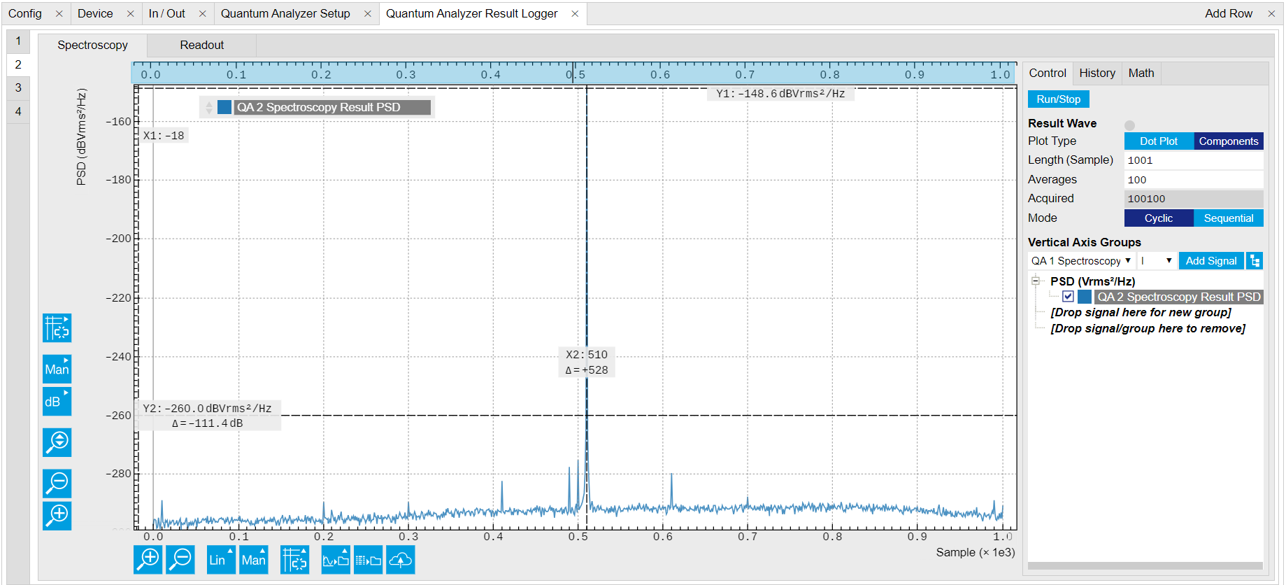
Figure 6: power spectral Density when input signal is ON on QA Result Logger Tab.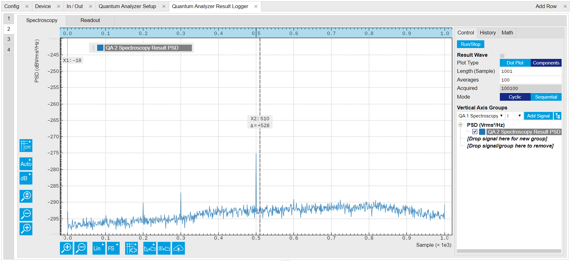

Figure 7: power spectral Density when input signal is OFF on QA Result Logger Tab.

Python API SHFSweeper class is the core of the power spectral density measurements. It defines all relevant parameters for frequency sweeping and sequencing. Toolkit wraps around the SHFSweeper and exposes an interface that is similar to the LabOne modules, meaning the parameters are exposed in a node tree like structure. The power spectral density of input signal is measured using the SHFQA+ Sweeper as for Resonator Spectroscopy Measurement with sweeper.sweep.psd(True).

By calculating square of measurement result after integration at different frequencies, the power spectral density at frequency \(f\) is \(S_{xx}(f) = \lim_{N\to\infty} \frac{(\Delta t)^2}{T}|\sum_{n = -N}^{n = N} x_ne^{-i2\pi f n\Delta t}|^2\), where \(\Delta t = 1/f_\mathrm{s}\) is the time step, \(f_\mathrm{s}\) is the sampling rate, \(T = (2N+1)\Delta t\) is the integration length in seconds, \(2N+1\) is the integration length in samples, \(x_n\) is the \(n\)-th complex data of the input signal, \(e^{-i2\pi f n\Delta t}\) is the integration weight. By sweeping the frequency of integration weight, the power spectral density of input signal is calculated by the instrument, and it returns the real-valued power spectral density in units of \(\mathrm{Vrms}^2/\mathrm{Hz}\).

Connect the Instrument

Create a toolkit session to the data server and connect the Instrument with the device ID, e.g. 'DEV12001', see Connecting to the Instrument.

# Load the LabOne API and other necessary packages
from zhinst.toolkit import Session

DEVICE_ID = 'DEVXXXXX'
SERVER_HOST = 'localhost'

session = Session(SERVER_HOST)              ## connect to data server
device = session.connect_device(DEVICE_ID)  ## connect to device

Create a Sweeper and configure it
```
sweeper = session.modules.shfqa_sweeper
sweeper.device(device)

# configure QA channel 2
CHANNEL_INDEX = 1 # physical Channel 2
sweeper.sweep.start_freq(-500e6) # in units of Hz
sweeper.sweep.stop_freq(500e6) # in units of Hz
sweeper.sweep.num_points(1001)
sweeper.average.num_averages(100)

sweeper.average.integration_time(10e-6) # in units of second
sweeper.sweep.wait_after_integration(1e-6) # waiting 1 us after integration before starting a new measurement 

sweeper.average.mode("cyclic") # "sequential" or "cyclic" averaging

sweeper.rf.channel(CHANNEL_INDEX)
sweeper.rf.center_freq(5e9) # in units of Hz
sweeper.rf.input_range(0) # in units of dBm
sweeper.sweep.psd(True)

device.qachannels[CHANNEL_INDEX].input.on(1)
```
The sweep parameters are configured such that the offset frequency of integration weight is linearly swept over 1001 points from -500 MHz to 500 MHz around the center frequency of 5 GHz with the input power range of 0 dBm and the oscillator gain of 0.5, the input signal is integrated for 10 μs after receiving a trigger, and the measurement is repeated 100 times.

There are 2 sweeping modes, sequencer-based mode (default) and host-driven mode. The sequencer-based mode is recommended to achieve the highest sweep speed. In the sequencer-based mode, the frequency sweep is done by updating the frequency of the digital oscillator via the SeqC commands configFreqSweep and setSweepStep. This mode allows a fast resonator spectroscopy measurement with predicted cycle time of \(t_{\mathrm{settling\ time}} + t_{\mathrm{integration\ delay}} + t_{\mathrm{integration\ time}} + t_{\mathrm{wait\ after\ integration}}\), see . In the host-driven mode, the frequency sweep is done by updating the frequency of the digital oscillator via software, therefore measurement speed is limited by communication between instrument and host computer. Logarithmic or other non-linear frequency sweep is supported by the host-driven sweep mode only.

To get a better signal-to-noise ratio (SNR), the measurement is repeated, and the result is averaged. There are 2 ways for averaging, sequential and cyclic. In the sequential mode, measurement is repeated after each frequency step. In the cyclic mode, measurement is repeated after sweeping through all frequencies.

Configure a signal under test

For simplicity, we generate a continuous waveform using Signal Output 4 with the following codes.

CHANNEL_INDEX_OUTPUT = 3 # Physical channel 4

with device.set_transaction():
    device.qachannels[CHANNEL_INDEX_OUTPUT].centerfreq(5e9) # center frequency in units of Hz
    device.qachannels[CHANNEL_INDEX_OUTPUT].output.range(0) # power range in units of dBm
    device.qachannels[CHANNEL_INDEX_OUTPUT].output.on(1) # turn on output 
    device.qachannels[CHANNEL_INDEX_OUTPUT].mode(0) # Spectroscopy mode
    device.qachannels[CHANNEL_INDEX_OUTPUT].oscs[0].gain(0.5) # amplitude factor of digital oscillator
    device.qachannels[CHANNEL_INDEX_OUTPUT].spectroscopy.envelope.enable(0) # continuos wave

Run the measurement and plot the data
```
psd = sweeper.run()
sweeper.plot()
```
After executing sweeper.run(), all above parameters are updated, and a SeqC program is automatically generated, uploaded and compiled based on the sweep parameters, see in . In the program, ConfigFreqSweep sets the start frequency and the frequency increment in units of Hz for a chosen oscillator, and setSweepStep sets the oscillator frequency. The oscillator phase is reset by resetOscPhase before each measurement. The trigger generated in the sequencer is used to start the integration, and the playZero sets the cycle duration. The measurement is repeated using the nested for loop according to the averaging mode. The measurement starts after enabling the sequencer.

Figure 8: Seqc program in the Readout Pulse Generator Tab.

The result returned from sweeper.run() is the power spectral density in units of \(\mathrm{Vrms}^2/\mathrm{Hz}\). It is averaged and normalized by the integration length. The sweeper.plot() converts the unit of power spectral density from \(\mathrm{Vrms}^2/\mathrm{Hz}\) to dBm/Hz by

\[ \begin{equation}\tag{1} \begin{aligned} P_{\mathrm{dBm/Hz}} & = 10\log(\frac{P_{\mathrm{Vrms}^2/\mathrm{Hz}}\times 1000}{R}), \end{aligned} \end{equation} \]

where \(R\) is 50 \(\Omega\), 1000 is the conversion factor from W to mW. The power spectral density in units of dBm/Hz is shown in Figure 9.

To remove the background noise from the instrument and environment repeat the measurement with Signal Output 4 is disabled.

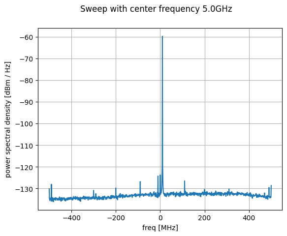
Figure 9: Power spectral density of signal from Signal Output 4.