HDAWG precompensation curve fit

Demonstrate how to use the precompensation module to fit filter parameters for a measured signal.

Requirements:

• LabOne Version >= 22.08

• Instruments: 1 x HDAWG Instrument

from zhinst.toolkit import Session
import numpy as np
from scipy import signal
from lmfit import Model

session = Session("localhost")
device = session.connect_device("DEVXXXX")

sampling_rate = device.system.clocks.sampleclock.freq(2.4e9, deep=True)

Generate target signal

MIN_X = -96
MAX_X = 5904
x_values = np.array(range(MIN_X, MAX_X))
x_values = [element / sampling_rate for element in x_values]
target_signal = np.array(np.concatenate((np.zeros(-MIN_X), np.ones(MAX_X))))

Generate actual signal

Generate “actual signal” through filtering the initial signal with an exponential filter and add noise.

TAU = 100e-9
AMPL = 0.4

# calculate a and b from amplitude and tau
alpha = 1 - np.exp(-1 / (sampling_rate * TAU * (1 + AMPL)))
if AMPL >= 0.0:
    k = AMPL / (1 + AMPL - alpha)
    signal_a = [(1 - k + k * alpha), -(1 - k) * (1 - alpha)]
else:
    k = -AMPL / (1 + AMPL) / (1 - alpha)
    signal_a = [(1 + k - k * alpha), -(1 + k) * (1 - alpha)]
signal_b = [1, -(1 - alpha)]

distorted_signal = np.array(
    signal.lfilter(signal_b, signal_a, target_signal)
    + 0.01 * np.random.normal(size=target_signal.size)
)

Prepare the Precompensation Advisor module

module = session.modules.precompensation_advisor
module.device(device)
# Manually load wave through the inputvector node.
module.wave.input.source("manual")
# Use a single exponential filter.
module.exponentials[0].enable(True)

Fitting the parameters

def labone_exponential_filter(module_handle, input_signal, amplitude, timeconstant):
    """Calculate precompensated signal for a single exponential filter.

    Uploads the input_signal to the precompensationAdvisor module and returns
    the simulated forward transformed signal with an exponential
    filter(amplitude,timeconstant).

    Args:
        module_handle: Precompensation Advisor Module.
        input_signal: Amplitude data used as a signal source.
        amplitude: Amplitude of the exponential filter.
        timeconstant: Time constant (tau) of the exponential filter.
    """
    module_handle.exponentials[0].amplitude(amplitude)
    module_handle.exponentials[0].timeconstant(timeconstant)
    module_handle.wave.input.inputvector(input_signal)
    return np.array(module_handle.wave.output.forwardwave()["x"])

model = Model(
    labone_exponential_filter, independent_vars=["module_handle", "input_signal"]
)
result = model.fit(
    target_signal,
    input_signal=distorted_signal,
    module_handle=module,
    amplitude=0.0,
    timeconstant=1e-4,
    fit_kws={"epsfcn": 1e-3},
)
# 'epsfcn' is needed as filter parameters are discretized in precompensationAdvisor
# module, otherwise fitting will not converge
print(result.fit_report())

[[Model]]
    Model(labone_exponential_filter)
[[Fit Statistics]]
    # fitting method   = leastsq
    # function evals   = 72
    # data points      = 6000
    # variables        = 2
    chi-square         = 0.30571694
    reduced chi-square = 5.0970e-05
    Akaike info crit   = -59303.6624
    Bayesian info crit = -59290.2634
[[Variables]]
    amplitude:     0.39604559 +/- 0.00115905 (0.29%) (init = 0)
    timeconstant:  1.0186e-07 +/- 3.8885e-10 (0.38%) (init = 0.0001)
[[Correlations]] (unreported correlations are < 0.100)
    C(amplitude, timeconstant) = -0.752

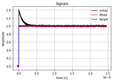
Plot results

import matplotlib.pyplot as plt

_, axis = plt.subplots()
axis.plot(x_values, result.init_fit, "k", label="initial")
axis.plot(x_values, result.best_fit, "r", label="fitted")
axis.plot(x_values, target_signal, "b", label="target")
axis.legend()
axis.ticklabel_format(axis="both", style="sci", scilimits=(-2, 2))
axis.set_xlabel("time [s]")
axis.set_ylabel("Amplitude")
plt.title('Signals')
plt.grid()
plt.show()