Synchronization of HDAWGs and UHFQA
Note
This tutorial is applicable to the PQSC when used with multiple HDAWG and UHFQA.
Goals and Requirements
The goal of this tutorial is to demonstrate the multi-HDAWG and UHFQA synchronization with the PQSC for signal generation and signal acquisition. We demonstrate how to synchronize the clock reference and triggers of all the instruments, how to synchronously start the signal generation and how to align with the signal acquisition. This tutorial assumes that you are already familiar with the PQSC and the HDAWG, otherwise, please follow first the tutorial for multi-HDAWG synchronization in Synchronization of multiple HDAWGs. In order to visualize the multi-channel signals, an oscilloscope with sufficient bandwidth and channel number is required.
The equipment list is given below.
- 1 PQSC
- 2 or more HDAWGs
- 1 UHFQA
- 1 External 10 MHz reference clock
- 1 oscilloscope (min. 4 channels, bandwidth 500 MHz or more)
- 1 Ethernet switch
- 1 Ethernet cable per instrument (supplied with your PQSC, HDAWGs and UHFQA)
- 1 ZSync cable per HDAWG (supplied with your HDAWGs)
- 1 DIO cable with level adapter (supplied with your UHFQA)
- 6 SMA coaxial cables
- 1 BNC coaxial cables
- 1 power splitter SMA for the reference clock
- 3 adaptors BNC male to SMA female
Preparation
Connect the cables as illustrated below. The cables connecting the 10 MHz reference clock to the PQSC and the UHFQA must have the same length. Make sure that the instruments are powered on and connected by Ethernet to your local area network (LAN) where the host computer resides.
For best performance, the system should be placed in a climate-controlled environment with stable temperature and humidity. Avoid exposing the instruments to direct sunlight.
After starting LabOne, the default web browser opens with the LabOne graphical user interface. It’s advised to open a tab in the browser for each instrument.

The tutorial can be started with the default instrument configuration (e.g. after a power cycle or after loading the Factory Default preset from the 'Device' tab) and the default user interface settings (e.g. as is after pressing F5 in the browser).
Note
The PQSC needs to warm-up for 30 minutes after power-up. Do not lock to external reference clock or start triggering before it’s ready. The CLK LED on the bottom right of the LabOne interface will turn green when the instrument is warmed up and ready to use.
Multi device synchronization
The first step to enable the device synchronization is to distribute the reference clocks to the instruments and enable the triggering. The PQSC and the UHFQA need an external 10 MHz reference clock, while the HDAWGs receive their reference clock over ZSync. It’s important to first enable the external reference clock on the PQSC and then on the HDAWGs/UHFQA, since a change of the clocking in the PQSC will cause a disconnection of the devices connected over ZSync. The following tables summarizes the necessary settings for each instrument.
| Tab | Sub-tab | Section | # | Label | Setting / Value / State |
|---|---|---|---|---|---|
| Device | Configuration | Reference clock Input Source | External |
| Tab | Sub-tab | Section | # | Label | Setting / Value / State |
|---|---|---|---|---|---|
| Device | Configuration | Reference clock Source | ZSync | ||
| Device | Configuration | Sample Clock Frequency (Hz) | 2.4G | ||
| DIO | Digital I/O | Mode | QCCS |
| Tab | Sub-tab | Section | # | Label | Setting / Value / State |
|---|---|---|---|---|---|
| Device | Configuration | Settings Clock Source | 10MHz |
On the PQSC and the HDAWGs, after changing the selector, the ‘Status’ LED will turn yellow for few seconds and then green again to signal that the instruments successfully locked to the reference clock.
Then, check that the PQSC correctly recognized the HDAWGs. On the back of the instrument or in the Ports tab of the PQSC verify that the status LED of the used ZSync ports turned blue and the serial number of the HDAWG is displayed. You may assign an alias to for each instrument to easily recognize it later. The UHFQA is not visible on the PQSC.
The next step is to enable the distribution of the triggers from the PQSC to the other instruments. The HDAWGs receive triggers over the ZSync port directly from the PQSC. The UHFQA receives them indirectly via the HDAWG over the DIO port. Here the HDAWG serves as a bridge to the PQSC. First we enable the interface; the following tables summarizes the necessary settings for the UHFQA and the HDAWG 2. The HDAWG 1 doesn’t need any further configuration since it has no UHFQA connected and thus does not have to operate as a bridge.
Note
When an HDAWG is used as bridge for the UHFQA, its sample rate must be 2.4 GSa/s. As consequence, also the other HDAWGs in the system must use this sample rate, since the sample rates 2.0 GSa/s and 2.4 GSa/s can’t be mixed.
| Tab | Sub-tab | Section | # | Label | Setting / Value / State |
|---|---|---|---|---|---|
| DIO | Digital I/O | Mode | Manual | ||
| DIO | Digital I/O | All | Drive | OFF | |
| DIO | Digital I/O | Clock | Internal 50 MHz |
| Tab | Sub-tab | Section | # | Label | Setting / Value / State |
|---|---|---|---|---|---|
| DIO | Digital I/O | Interface | LVCMOS | ||
| DIO | Digital I/O | 31...24 | Drive | ON | |
| DIO | Digital I/O | 23...16 | Drive | ON | |
| DIO | Digital I/O | 15...8 | Drive | OFF | |
| DIO | Digital I/O | 7...0 | Drive | OFF |

Next, the AWG sequencer on the UHFQA needs to be configured with the right DIO trigger signal assignment. A complete description of the signals on the DIO port can be found in the HDAWG or UHFQA manuals. The following table summarizes the correct assignments for this tutorial.
| Tab | Sub-tab | Section | # | Label | Setting / Value / State |
|---|---|---|---|---|---|
| AWG | Trigger | DIO Trigger | Strobe Slope | None | |
| AWG | Trigger | DIO Trigger | Valid Index | 16 | |
| AWG | Trigger | DIO Trigger | Valid Polarity | High |
Now all the sequencers are ready to receive triggers issued by the PQSC synchronously.
Multi device signal generation
We configure the AWG sequencers to play a square waveform as soon as the trigger from the PQSC is received. The necessary settings are summarized in the following tables.
| Tab | Sub-tab | Section | # | Label | Setting / Value / State |
|---|---|---|---|---|---|
| Output | Waveform Generators | 4x2 channels | |||
| Output | Waveform Generators | 1 | Output Amplitude Wave 1 | 1.0 | |
| Output | Waveform Generators | 1 | Modulation | OFF | |
| Output | Wave Outputs | 1 | Range | 2 V | |
| Output | Wave Outputs | 1 | On | ON |
| Tab | Sub-tab | Section | # | Label | Setting / Value / State |
|---|---|---|---|---|---|
| In / Out | Signal Outputs | 2 | 50 Ω | ON | |
| In / Out | Signal Outputs | 2 | Range | 750 mV | |
| In / Out | Signal Outputs | 2 | On | ON | |
| AWG | Control | Rerun | OFF | ||
| AWG | Control | Output 2 | Amplitude (FS) | 1.0 | |
| AWG | Control | Output 2 | Mode | Plain |
The following sequence programs should be loaded in the sequencers and then started. For the UHFQA:
const WAVE_GRANULARITY_UHFQA = 24;
wave w = ones(WAVE_GRANULARITY_UHFQA*2);

while(true) {
  waitZSyncTrigger();
  playWave(2, w);
}
And for the HDAWG:
const WAVE_GRANULARITY_HDAWG = 32;
wave w = 0.75*ones(WAVE_GRANULARITY_HDAWG*2);

while(true) {
  waitZSyncTrigger();
  playWave(w);
}
The AWG status LED will turn yellow, meaning that is ready and waiting
for the trigger. Configure the scope as described in
Synchronization of multiple HDAWGs.
Finally, we configure the periodic trigger generation in the Ports tab
of the PQSC and then start it by clinking on the  button.
| Tab | Sub-tab | Section | # | Label | Setting / Value / State |
|---|---|---|---|---|---|
| Ports | Control | Repetitions | 2 | ||
| Ports | Control | Holdoff (s) | 100n |
On the scope we can now see two identical pulses with both channels aligned in time. The inter-channel alignment can be further adjusted by changing the delay of the HDAWG Wave output in the field "Output > Wave Outputs > Delay (s)".
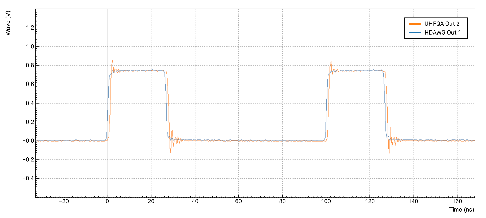
To obtain two identical pulses we had to adjust both the wave amplitude and range as well as the pulse length. The HDAWG range is the peak-to-peak voltage, while the UHFQA range is defined as the peak voltage, so there is factor of 2 to take into account. In the tutorial the waveform amplitude has been selected to be exactly 750 mV.
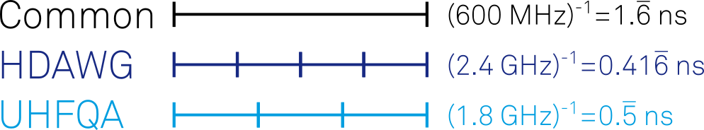
The sample rate of the two instruments are different, 2.4 GSa/s for the HDAWG and 1.8 GSa/s for the UHFQA. The common frequency is 600 MHz, so approximately every 1.66 ns they align. In other words, two channels align respectively every 4 samples and 3 samples, as shown in this sketch
The waveform granularity is 16 samples on the HDAWG and 8 samples on the
UHFQA. If we design our sequence programs such that they respect a
waveform granularity of 32 samples on the HDAWG and 24 samples on the
UHFQA, the output will be always aligned. In units of time, this
correspond to a granularity of approximately 13.33 ns. The waveform
playback instruction playWave should follow immediately after the
instruction waitZSyncTriggger() to ensure the alignment. The playback
should be also gapless, so it’s necessary to avoid long wait
instructions or too short waveform in complex loops.
To introduce efficient spacers, it’s possible to use the playZero
instruction. The length of the spacer pulse should respect the same
granularity rules and match the length of the pulses played on the other
instruments. For example, if in the previous example we want the pulses
to occur one after the other, we can modify the UHFQA sequence program
as follow:
const WAVE_GRANULARITY_UHFQA = 24;
wave w = ones(WAVE_GRANULARITY_UHFQA*2);

while(true) {
  waitZSyncTrigger();
  playZero(WAVE_GRANULARITY_UHFQA*2);
  playWave(2, w);
}

Multi-device signal generation and acquisition
The loopback connection on the UHFQA can be used to simulate the response of the device under test. In this example we use a single PQSC trigger to mark the start, the timing of the following signals will be controlled by the sequencers on the HDAWGs and the UHFQA. We simulate a simple experiment where a generic drive pulse is generated by the HDAWG. This pulse is immediately followed by a readout pulse generated by the UHFQA, which is also triggered for the readout. The control pulse is modulated at 150 MHz and the readout pulse is modulated at 50 MHz. Signal input 1 of the UHFQA is used to acquire the signal. The holdoff time is increased, so the PQSC will be running during the play of all the waveforms. Configure the PQSC as follows:
| Tab | Sub-tab | Section | # | Label | Setting / Value / State |
|---|---|---|---|---|---|
| Ports | Control | Repetitions | 1 | ||
| Ports | Control | Holdoff (s) | 1m |
The following sequence programs should be uploaded to the AWG sequencers and then started. For the UHFQA:
// Constants declaration
const WAVE_GRANULARITY_UHFQA = 24;
const DRIVE_PULSE_LEN = WAVE_GRANULARITY_UHFQA*5;
const READOUT_LEN = WAVE_GRANULARITY_UHFQA*10;
const PAD_LEN = WAVE_GRANULARITY_UHFQA*50;
const READOUT_FREQ = 50e6;
const AVERAGES = 1024;

// Waveform declaration
wave w_sine = sine(READOUT_LEN, 0, READOUT_FREQ*READOUT_LEN/DEVICE_SAMPLE_RATE);

// Execution
var i;
while(true) {
  waitZSyncTrigger();
  for (i = 0; i < AVERAGES; i++) {
    playZero(DRIVE_PULSE_LEN);

    playWave(1, w_sine, 2, w_sine);
    // Trigger the readout
    startQA(QA_INT_ALL, true);

    playZero(PAD_LEN);
  }
}
And for the HDAWG:
// Constants declaration
const WAVE_GRANULARITY_HDAWG = 32;
const DRIVE_PULSE_LEN = WAVE_GRANULARITY_HDAWG*5;
const READOUT_LEN = WAVE_GRANULARITY_HDAWG*10;
const PAD_LEN = WAVE_GRANULARITY_HDAWG*50;
const DRIVE_FREQ = 150e6;
const AVERAGES = 1024;

// Waveform declaration
wave w_drive = cosine(DRIVE_PULSE_LEN, 0, DRIVE_FREQ*DRIVE_PULSE_LEN/DEVICE_SAMPLE_RATE);
w_drive *= gauss(DRIVE_PULSE_LEN, DRIVE_PULSE_LEN/2, DRIVE_PULSE_LEN/6);

// Execution
var i;
while(true) {
  waitZSyncTrigger();
  for (i = 0; i < AVERAGES; i++) {
    playWave(w_drive);

    playZero(READOUT_LEN);
    // Trigger the readout (on the UHFQA)
    //startQA(QA_INT_ALL, true);

    playZero(PAD_LEN);
  }
}
The UHFQA sequence generates a trigger signal to start the QA Weighted Integration unit and the QA Input Monitor. While the command to generate such trigger may look like a violation of the rule to have identical gapless sequences, it’s indeed still valid. The execution time of these instructions is approximately 4 clock cycles of the sequencer, significantly less then the length of the previous waveform. The sequencer has enough time to do that while playing the first waveform, so the playback is gapless and the equal timing on the sequencers is respected. In order to trigger correctly the readout, we have to configure the integration unit in accordance with the generated signal:
| Tab | Sub-tab | Section | # | Label | Setting / Value / State |
|---|---|---|---|---|---|
| QA Setup | Integration | Mode | Standard | ||
| QA Setup | Integration | Length | 240 | ||
| QA Setup | Integration | Trigger Signal | AWG Integration Trigger |
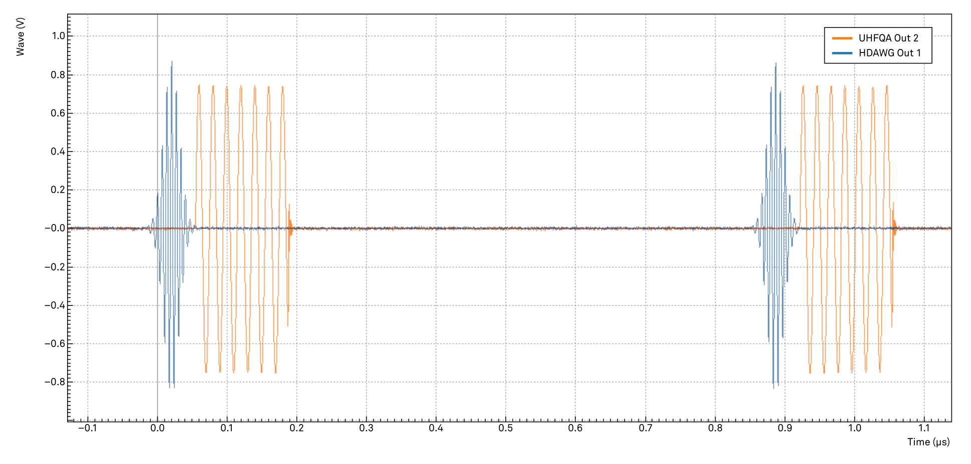
The generated signal shows two modulated pulses aligned in time. In contrast to the previous example, the two-fold repetition of the pulses is controlled by loops in the sequence programs and not by the periodic trigger generation on the PQSC.
To acquire the time trace of the signal on the channel 1 we have to configure the UHFQA as follows:
| Tab | Sub-tab | Section | # | Label | Setting / Value / State |
|---|---|---|---|---|---|
| In / Out | Signal Outputs | 1 | 50 Ω | ON | |
| In / Out | Signal Outputs | 1 | Range | 750 mV | |
| In / Out | Signal Outputs | 1 | On | ON | |
| AWG | Control | Output 1 | Amplitude (FS) | 1.0 | |
| AWG | Control | Output 1 | Mode | Plain | |
| QA Setup | Deskew | Delay (Sample) | 192 | ||
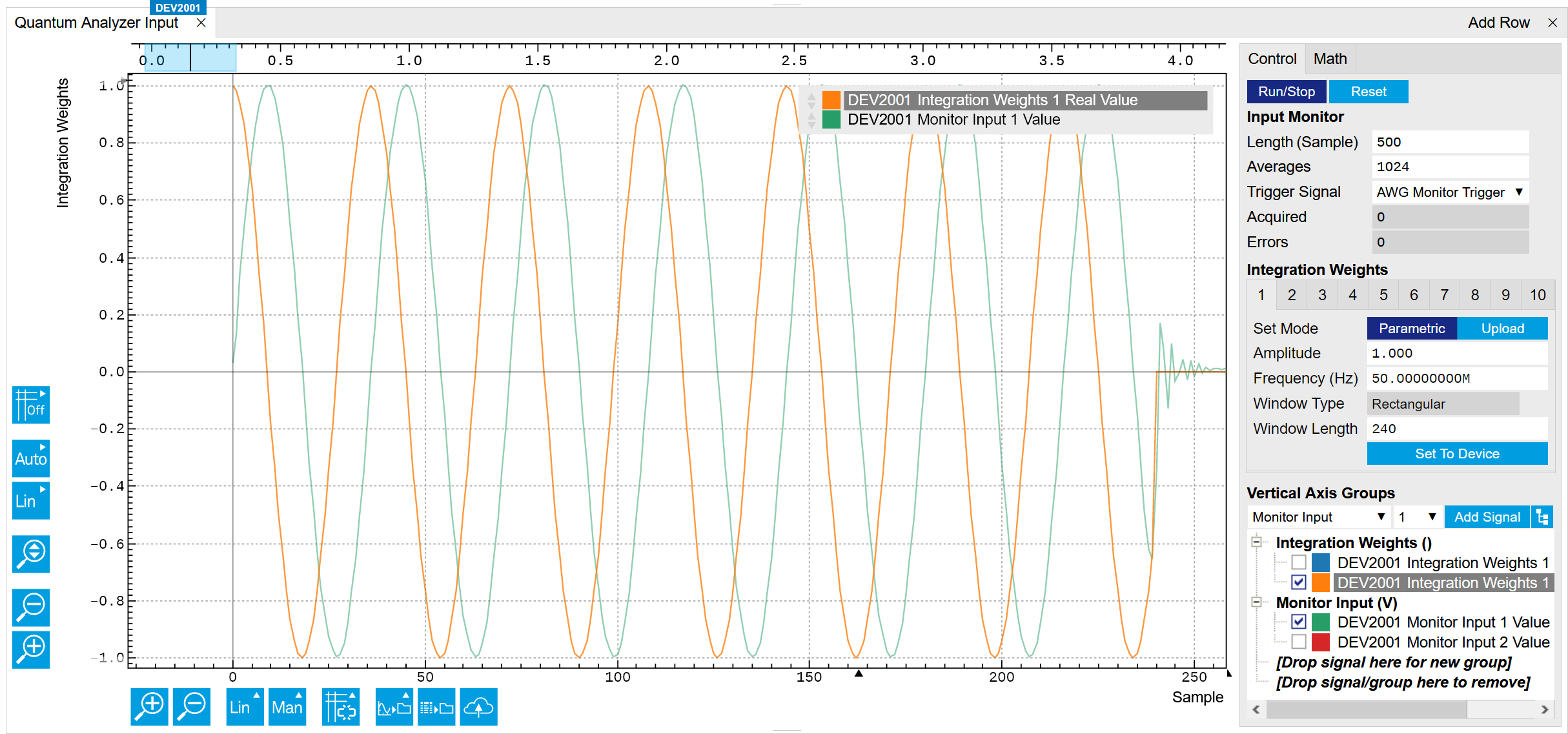
| QA Input | Control | Input Monitor | Length (Sample) | 500 | |
| QA Input | Control | Input Monitor | Averages | 1024 | |
| QA Input | Control | Run/Stop | click | ||
| QA Input | Control | Reset | click |
When the PQSC trigger is sent again, we can observe that the QA Input Monitor gets triggered by the sequencer. It acquires and averages all the 1024 pulses. The trigger and the pulses are correctly aligned since they average out all correctly, otherwise the signal would have been distorted. The alignment can be further adjusted with the Delay setting in the QA Setup tab, the value given in this tutorial is for a very short loopback cable.
The Monitor is good to visualize the pulses, but for the real acquisition we need to configure the integration unit to demodulate our signal. We will demodulate the signal only on channel 1, like in a typical lock-in measurement. Configure the QA as follows and start the PQSC trigger again.
| Tab | Sub-tab | Section | # | Label | Setting / Value / State |
|---|---|---|---|---|---|
| QA Setup | Integration | 1 | Signal Input Mapping | 1→ Real, 1→ Imag | |
| QA Input | Control | Weights / Generate | Amplitude | 1 | |
| QA Input | Control | Weights / Generate | Frequency | 50 M | |
| QA Input | Control | Weights / Generate | Window Length | 240 | |
| QA Input | Control | Weights / Generate | Channel | 1 | |
| QA Input | Control | Weights / Generate | Set | click | |
| QA Result | Control | Result Wave | Source | Integration | |
| QA Result | Control | Result Wave | Length (Sample) | 1024 | |
| QA Result | Control | Result Wave | Averages | 1 | |
| QA Result | Control | Run/Stop | click | ||
| QA Result | Control | Reset | click |
All 1024 results are identical up to the noise, as is evident from the scatter plot in the complex plane shown in Figure 8.

In this case, the acquired value is approximately \(0.021 + 89.34i\), which is compatible with the expected value \(0 + 90i = A/2⋅N\), where \(A\) is the peak amplitude of the acquired signal (750 mV) and \(N\) is the number of acquired points (240). The signal is all in quadrature because we are generating a signal all in quadrature (sine instead of cosine). For more details, please refer to the UHFQA User Manual