Spectrum Analyzer Tab

The Spectrum Analyzer is one of the powerful frequency domain measurement tools introduced in Unique Set of Analysis Tools and is available on all GHFLI instruments.

Features

Fast, high-resolution FFT spectrum analyzer
Signals: demodulated data (X+iY, R, Θ, f and dΘ/dt/(2π) ), and more
Variable center frequency, frequency resolution and frequency span
Auto bandwidth
Waterfall display
Choice of 4 different FFT window functions
Continuous and block-wise acquisition with different types of averaging
Detailed noise power analysis
Mathematical toolbox for signal analysis

Description

The Spectrum Analyzer provides frequency domain analysis of demodulator data. Whenever the tab is closed or an additional one of the same type is needed, clicking the following icon will open a new instance of the tab.

Table 1. App icon and short description
Control/Tool	Option/Range	Description
Spectrum		Provides FFT functionality to all continuously streamed measurement data.

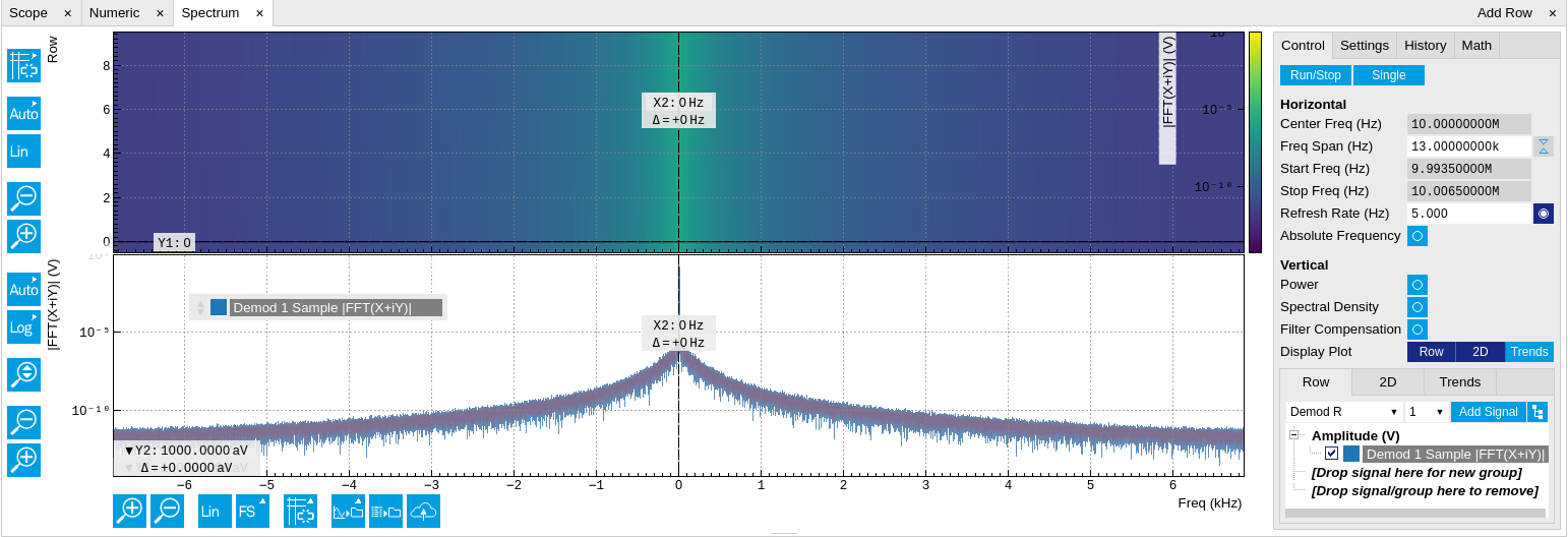
The Spectrum tab (see Figure 1) is divided into a display section on the left and a configuration section on the right. The configuration section is further divided into a number of sub-tabs.

Figure 1. LabOne UI: Spectrum analyzer tab

The Spectrum Analyzer allows for spectral analysis of all the demodulator data by performing a fast Fourier transform (FFT) on the complex demodulator data samples X+iY (where i is the imaginary unit). The result of this FFT is a spectrum centered around the demodulation frequency, whereas applying a FFT directly on the raw input data would produce a spectrum centered around zero frequency. The latter procedure corresponds to the Frequency Domain operation in the Scope Tab . The main difference between the two is that the Spectrum Analyzer tool can acquire data for a much longer periods of time and therefore can achieve a very high frequency resolution around the demodulation frequency.

By default, the display section contains a line plot of the spectrum together with a color waterfall plot of the last few acquired spectra. The waterfall plot makes it easier to see the evolution of the spectrum over time. The display layout as well as the number of rows in the color plot can be configured in the Settings sub-tab.

Data shown in the Spectrum tab have passed through a low-pass filter with a well-defined order and bandwidth. This is most clearly visible in the shape of the noise floor. One has to take care that the selected frequency span, which equals the demodulator sampling rate, is 5 to 10 times higher than the filter bandwidth in order to prevent measurement errors due to aliasing. The Auto Bandwidth button btn uielements A um adjusts the sampling rate so that it suits the filter settings. The Spectrum tab features FFT display of a selection of data available in the Signal Type drop-down list in addition to the complex demodulator samples X+iY. Looking at the FFT of polar demodulator values R and Theta allows one to discriminate between phase noise components and amplitude noise components in the signal. The FFT of the phase derivative dΘ/dt provides a quantitative view of the spectrum of demodulator frequencies. Note that many of the signals in the Signal Type list are real-valued, rather than complex-valued. Their spectra are single-sided with minimum frequency of 0 Hz.

Functional Elements

Table 2. Spectrum tab: Settings sub-tab
Control/Tool	Option/Range	Description
Run/Stop		Run the FFT spectrum analysis continuously
Single		Run the FFT spectrum analysis once
Frequency Span (Hz)	numeric value	Set the frequency span of interest for the complex FFT. A FFT based on real input data will display half of the frequency span up to the Nyquist frequency.
Refresh Rate (Hz)	numeric value	Set the maximum plot refresh rate. The actual refresh rate also depends on other parameters such as FFT length. In overlapped mode the refresh rate defines the amount of overlapping.
Power	ON / OFF	Calculate and show the power value. To extract power spectral density (PSD) this button should be enabled together with spectral density.
Spectral Density	ON / OFF	Calculate and show the spectral density. If power is enabled the power spectral density value is calculated. The spectral density is used to analyze noise.
Filter Compensation	ON / OFF	Spectrum is corrected by demodulator filter transfer function. Allows for quantitative comparison of amplitudes of different parts of the spectrum.
FFT length	numeric value	The number of samples used for the FFT. Values entered that are not a binary power are truncated to the nearest power of 2.
Sampling Progress	0% to 100%	The percentage of the FFT buffer already acquired. The progress includes the number of rows and averages.
FFT Duration (s)	numeric value	Indicates the length in time of the samples used for a single FFT.
Window	Rectangular	Several different FFT windows to choose from. Depending on the application it makes a huge difference which of the provided window function is used. Please check the literature to find out the best trade off for your needs.
	Hann
	Hamming
	Blackman Harris
	Flat Top
	Exponential (ring-down)
	Cosine (ring-down)
	Cosine squared (ring-down)
Resolution (Hz)	mHz to Hz	Spectral resolution defined by the reciprocal acquisition time (sample rate, number of samples recorded).
Rows	numeric value	Number of rows
Averages	numeric value	Number of FFT averaged for each row. Setting the value to 1 will disable any averaging.
Waterfall	ON / OFF	Enable to show the 2D plot in waterfall mode. It will always update the lowest line.
Overwrite	ON / OFF	Enable to overwrite the grid in continuous mode. History will not be collected. A history element will only be created when the analysis is stopped.
Plot Type		Select the plot type.
	None	No plot displayed.
	2D	Display defined number of grid rows as one 2D plot.
	Row	Display only the trace of index defined in the Active Row field.
	2D + Row	Display 2D and row plots.
Active Row	integer value	Set the row index to be displayed in the Row plot.
Track Active Row	ON / OFF	If enabled, the active row marker will track with the last recorded row. The active row control field is read-only if enabled.
Palette	Viridis	Select the colormap for the current plot.
	Inferno
	Balance
	Turbo
	Grey
	Solar
Colorscale	ON / OFF	Enable/disable the colorscale bar display in the 2D plot.
Mapping		Mapping of colorscale.
	Lin	Enable linear mapping.
	Log	Enable logarithmic mapping.
	dB	Enable logarithmic mapping in dB.
Scaling	Full Scale/Manual/Auto	Scaling of colorscale.
Clamp To Color	ON / OFF	When enabled, grid values that are outside of defined Min or Max region are painted with Min or Max color equivalents. When disabled, Grid values that are outside of defined Min or Max values are left transparent.
Start	numeric value	Lower limit of colorscale. Only visible for manual scaling.
Stop	numeric value	Upper limit of colorscale. Only visible for manual scaling.

For the Math sub-tab please see the table "Plot math description" in the section called "Cursors and Math".