Scope Tab
The Scope is a powerful time domain and frequency domain measurement tool as introduced in Unique Set of Analysis Tools and is available on all GHFLI instruments.
Features
- Two input channels
- 14 bit nominal resolution
- Fast Fourier Transform (FFT): up to 2 GHz span (800 MHz in baseband), spectral density and power conversion, choice of window functions
Description
The Scope tab serves as the graphical display for time domain data. Whenever the tab is closed or an additional one of the same type is needed, clicking the following icon will open a new instance of the tab.
| Control/Tool | Option/Range | Description |
|---|---|---|
| Scope | Displays shots of data samples in time and frequency domain (FFT) representation. |
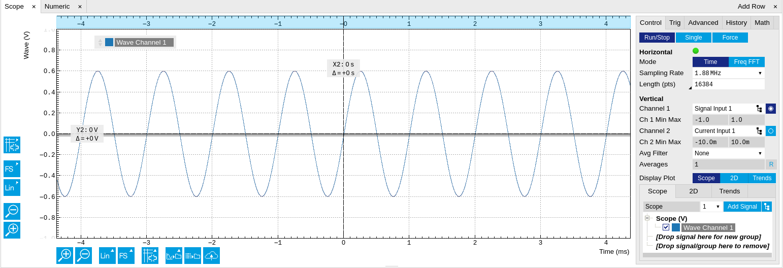
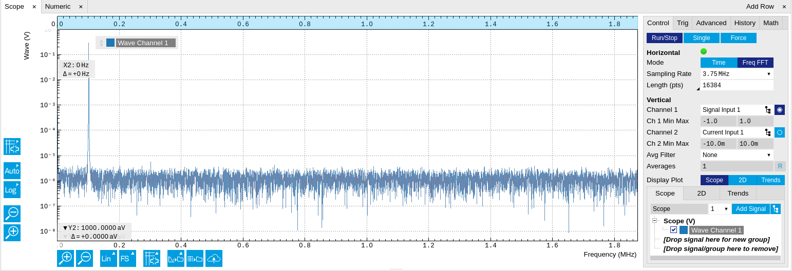
The Scope tab consists of a plot section on the left and a configuration section on the right. The configuration section is further divided into a number of sub-tabs. It gives access to a single-channel oscilloscope that can be used to monitor a choice of signals in the time or frequency domain. Hence the X axis of the plot area is time (for time domain display, Figure 1) or frequency (for frequency domain display, Figure 2). It is possible to display the time trace and the associated FFT simultaneously by opening a second instance of the Scope tab.
The Scope records data from a single channel at up to 4 GSa/s. The channel can be selected among the two Signal Inputs. The Scope records data sets of up to 524'288 samples.
The product of the inverse sampling rate and the number of acquired points (Length) determines the total recording time for each shot. Hence, longer time intervals can be captured by reducing the sampling rate.
The frequency domain representation is activated in the Control sub-tab by selecting Freq Domain FFT as the Horizontal Mode. It allows the user to observe the spectrum of the acquired shots of samples. All controls and settings are shared between the time domain and frequency domain representations.
The Scope supports averaging over multiple shots. The functionality is implemented by means of an exponential moving average filter with configurable filter depth. Averaging helps to suppress noise components that are uncorrelated with the main signal. It is particularly useful in combination with the Frequency Domain FFT mode where it can help to reveal harmonic signals and disturbances that might otherwise be hidden below the noise floor.
The Trigger sub-tab offers all the controls necessary for triggering on different signal sources. When the trigger is enabled, then oscilloscope shots are acquired whenever the trigger conditions are met. Trigger and Hysteresis levels can be indicated graphically in the plot. A disabled trigger is equivalent to continuous oscilloscope shot acquisition.
Functional Elements
| Control/Tool | Option/Range | Description |
|---|---|---|
| Single |  |
Acquires a single shot of samples. |
| Channel 1/2 |  |
Selects the signal source for the corresponding scope channel. Navigate through the tree view that appears and click on the required signal. Note: Channel 2 requires the DIG option. |
| Enable | ON / OFF | Activates the display of the corresponding scope channel. Note: Channel 2 requires the DIG option. |
| Run/Stop |  |
Runs the scope/FFT continuously. |
| Mode | Freq Domain (FFT) | Switches between time and frequency domain display. |
| Time Domain | ||
| Sampling Rate | 916 Sa/s to 60 MSa/s | Defines the sampling rate of the scope. The numeric values are rounded for display purposes. The exact values are equal to the base sampling rate divided by 2^n, where n is an integer. |
| Sampling Rate | Defines the sampling rate of the scope. The numeric values are rounded for display purposes. The exact values are equal to the base sampling rate divided by 2^n, where n is an integer. Warning: Due to the lack of sample averaging feature, reduced sampling rates can cause aliasing and thus artifacts in the signal spectrum. Currently, the Scope tool only supports sample decimation, but in the future it will also offer sample averaging. | |
| Average Filter | Enable Exponential Moving Average (EMA) filter that is applied when the average of several scope shots is computed and displayed. Depending on the mode, the source data for averaging is either the Time or the Freq FFT trace. | |
| Off | Averaging is turned off. | |
| On | Consecutive scope shots are averaged with an exponential weight. | |
| Averages | integer value | The number of shots required to reach 63% settling. Twice the number of shots yields 86% settling. |
| Reset |  |
Resets the averaging filter. |
For the Vertical Axis Groups, please see the table "Vertical Axis Groups description" in the section called "Vertical Axis Groups".
| Control/Tool | Option/Range | Description |
|---|---|---|
| Enable | ON / OFF | When triggering is enabled scope data are acquired every time the defined trigger condition is met. If disabled, scope shots are acquired continuously. |
| Segments | 1 to 32768 | Specifies the number of segments to be recorded in device memory. The maximum scope shot size is given by the available memory divided by the number of segments. This functionality requires the DIG option. |
| Shown Trigger | integer value | Displays the number of triggered events since last start. |
| Control/Tool | Option/Range | Description |
|---|---|---|
| FFT Window | Cosine squared (ring-down) | Several different FFT windows to choose from. Each window function results in a different trade-off between amplitude accuracy and spectral leakage. Please check the literature to find the window function that best suits your needs. |
| Rectangular | ||
| Hann | ||
| Hamming | ||
| Blackman Harris | ||
| Flat Top | ||
| Exponential (ring-down) | ||
| Cosine (ring-down) | ||
| Resolution (Hz) | mHz to Hz | Spectral resolution defined by the reciprocal acquisition time (sample rate, number of samples recorded). |
| Correction | ON / OFF | When Power is selected, it applies power correction to the spectrum to compensate for the shift that the window function causes. Power correction is useful for noise measurements to correct the noise floor. When Amp is selected, amplitude compensation is applied which corrects the peak amplitudes of coherent tones. |
| Absolute Frequency | ON / OFF | Shifts x-axis labeling to show the absolute frequency in the center as opposed to 0 Hz, when turned off. |
| Spectral Density | ON / OFF | Calculate and show the spectral density. If power is enabled the power spectral density value is calculated. The spectral density is used to analyze noise. |
| Power | ON / OFF | Calculate and show the power value. To extract power spectral density (PSD) this button should be enabled together with Spectral Density. |
| Persistence | ON / OFF | Keeps previous scope shots in the display. The color scheme visualizes the number of occurrences at certain positions in time and amplitude by a multi-color scheme. |
| Rate | Streaming rate of the scope channels. The streaming rate can be adjusted independent from the scope sampling rate. The maximum rate depends on the interface used for transfer. Note: scope streaming requires the DIG option. |
| Control/Tool | Option/Range | Description |
|---|---|---|
| History | History | Each entry in the list corresponds to a single trace in the history. The number of traces displayed in the plot is limited to 20. Use the toggle buttons to hide or show individual traces. Use the color picker to change the color of a trace in the plot. Double click on a list entry to edit its name. |
| Length | integer value | Maximum number of records in the history. The number of entries displayed in the list is limited to the 100 most recent ones. |
| Edit | Rename record. | |
| Delete | Remove record from the history list. | |
| Toggle all | Toggle all history traces. | |
| Clear All | Remove all records from the history list. | |
| Load file | Load data from a file into the history. Loading does not change the data type and range displayed in the plot, this has to be adapted manually if data is not shown. | |
| Name | Enter a name which is used as a folder name to save the history into. An additional three digit counter is added to the folder name to identify consecutive saves into the same folder name. | |
| Auto Save | Activate autosaving. When activated, any measurements already in the history are saved. Each subsequent measurement is then also saved. The autosave directory is identified by the text "autosave" in the name, e.g. "sweep_autosave_001". If autosave is active during continuous running of the module, each successive measurement is saved to the same directory. For single shot operation, a new directory is created containing all measurements in the history. Depending on the file format, the measurements are either appended to the same file, or saved in individual files. For HDF5 and ZView formats, measurements are appended to the same file. For MATLAB and SXM formats, each measurement is saved in a separate file. | |
| File Format | Select the file format in which to save the data. | |
| Save |  |
Save the traces in the history to a file accessible in the File Manager tab. The file contains the signals in the Vertical Axis Groups of the Control sub-tab. |
For the Math sub-tab please see the table "Plot math description" in the section called "Cursors and Math".