Characterizing a Two-Qubit System
Note
This tutorial is applicable to all SHFSG+ Instruments. A PQSC instrument is used in this tutorial to synchronize the output channels of the SHFSG+.
Note
Users can download all LabOne API Python example files from Github, https://github.com/zhinst/labone-api-examples.
Goals and Requirements
In this tutorial, the SHFSG+ is used to generate pulse sequences for characterizing a two-qubit system. We implement the pulse sequences using the Python API to measure the lifetimes of the two qubits, and to demonstrate how to perform Rabi, Ramsey and qubit spectroscopy measurements.
To visualize the generated output signals of the SHFSG+, an oscilloscope with sufficient bandwidth and at least 3 channels is required.
Preparation
Connect the cables as illustrated below. The first step to enable the device synchronization is to connect the SHFSG+ to a PQSC using both a ZSync port and the reference clock of the PQSC, as shown in Figure 1. For this we need to enable the ZSync clock and triggers on the SHFSG+.
Note
The synchronization and triggering of the SHFSG+ output channels can also be realized through an external trigger source connected to the trigger input connectors on the front panel of the SHFSG+.

The following tables summarizes the necessary settings for each instrument.
| Tab | Section | Label | Setting / Value / State |
|---|---|---|---|
| Device | Configuration | Reference clock Input | Internal |
| Device | Configuration | Reference clock Output | Enable |
| Device | Configuration | Reference clock Output Frequency | 100 MHz |
| Tab | Section | Label | Setting / Value / State |
|---|---|---|---|
| Device | Configuration | Input Reference Clock Set Source | External |
We will also monitor the SHFSG+ outputs using two channels of an external scope, and use a third scope channel for visualizing the marker output. Connect the outputs of the SHFSG+ to the oscilloscope as follows:
The following table summarizes the settings used to configure the external scope.
| Scope Setting | Value / State |
|---|---|
| Ch1-3 enable | ON |
| Ch1-2 range | 0.2 V/div |
| Timebase | 1 \(\mu\)s/div |
| Trigger source | Ch3 |
| Trigger level | 100 mV |
| Run / Stop | ON |
We also configure the FFT settings on the scope.
| Scope Setting | Value / State |
|---|---|
| Acquisition Time | 10 us |
| FFT Center | 1 GHz |
| FFT Span | 2 GHz |
Make sure that the instrument is powered on and connected by Ethernet to your local area network (LAN) in which the control computer resides. After starting LabOne, the default web browser opens with the LabOne graphical user interface. The tutorial can be started with the default instrument configuration (e.g. after a power cycle) and the default user interface settings (e.g. after pressing F5 in the browser). Additionally, this tutorial requires the use of one of our APIs, in order to perform the two qubit characterization measurements. We advise the user to ensure that the version of the LabOne Python API, LabOne and Firmware of the SHFSG+ device are updated and compatible . The examples shown here use the Python API. Similar functionality is available also for C+, Matlab and .Net, among others.
Qubit characterization set up
This tutorial describes how to perform various characterization measurements for a two superconducting qubit system using the measurement set up shown in Figure 2. For this, two control lines (green) are used to generate two qubits control pulses at microwave frequencies using Outputs 1 & 2 of the SHFSG+. To gain information about the state of the two qubits without directly interacting with them, dispersive readout resonators are used to probe the state of each qubit. Synchronization between the two instruments is ensured through the PQSC, which distributes its reference clock to both the SHFSG+ and the SHFQA+ through the ZSync link.
Upon a receiving the trigger signal from the PQSC, the two qubit control signals (green) are generated by the SHFSG+, followed by the multiplexed readout of the two qubits (purple) which is performed by the SHFQA+ in the readout mode. The readout results are then fed back to the PQSC for further processing.
Note
Each qubit is dispersively coupled to a readout resonator. Upon detecting the rising edge of a trigger from the PQSC, the SHFQA+ determines the state of the qubits (|g> ground or |e> excited states) by detecting any changes in the amplitudes and/or phases of the multiplexed microwave readout pulses, which probe the transmissions of the two resonators at frequencies \(f_{\mathrm{Res1}}\) and \(f_{\mathrm{Res2}}\).
Note
This tutorial can also be used to address other quantum systems, such as spin qubits, color centers, or neutral atoms, although some changes might be needed.

General Instruments configuration
In this section, we discuss the instrument configuration for the SHFSG+ channels using the LabOne Python API:
First we connect to the SHFSG+ using Python. For this we first create a
session with the Zurich Instruments Toolkit and then connect to the
instrument using the following code and by replacing DEVXXXXX with the
id of our SHFSG+ instrument, e.g. DEV12001:
## Load the LabOne API and other necessary packages
from zhinst.toolkit import Session
import numpy as np

DEVICE_ID = 'DEVXXXXX'
SERVER_HOST = 'localhost'

session = Session(SERVER_HOST)              ## connect to data server
device = session.connect_device(DEVICE_ID)  ## connect to device
Next we define the various output parameters of the SHFSG+ (e.g. center
frequency, power range). The NUMBER_OF_QUBITS parameter, which in this
case corresponds to 2 qubits, defines the number of channels used by the
SHFSG+. In this case, channel indices 0 & 1 are used, corresponding to
channels 1 & 2 on the front panel.
For both channels, the central frequency is set to 1 GHz, the output power range is fixed at 10 dBm, and all node settings are uploaded to the device using a transactional set.
## Define parameters for each SG channel
NUMBER_OF_QUBITS = 2
SGCHANNEL_NUMBER = [0,1]
SGCHANNEL_CENTER_FREQUENCY = [1e9,1e9]
SGCHANNEL_POWER_OUT = [10,10]
SGCHANNEL_TRIGGER_INPUT = 1

## configure sg channels
with device.set_transaction():
    for qubit in range(NUMBER_OF_QUBITS):
        print(SGCHANNEL_NUMBER[qubit],int(np.floor(SGCHANNEL_NUMBER[qubit]/2))+1)
        device.sgchannels[SGCHANNEL_NUMBER[qubit]].output.on(1)
        device.sgchannels[SGCHANNEL_NUMBER[qubit]].output.range(SGCHANNEL_POWER_OUT)
        synth = device.sgchannels[SGCHANNEL_NUMBER[qubit]].synthesizer()
        device.synthesizers[synth].centerfreq(SGCHANNEL_CENTER_FREQUENCY[qubit])
Qubit spectroscopy
The first experiment we describe is a qubit spectroscopy measurement, in which the frequencies of the control signals (green lines) for the two qubits are swept in parallel. A readout pulse (blue line) determines the qubit state for each frequency step of the control pulse.
In order to program the frequency sweep on both channels 1 & 2 of the
SHFSG+, we first need to define the parameters of the sweep by setting
the number of frequency steps (NUM_SWEEP_STEPS_QUBIT_SPECTROSCOPY) and
the integration time for the readout signal for each qubit. Then, we
also define the minimum/maximum frequencies of the sweep to be -100/300
MHz and -100/200 MHz for channels 1 & 2, respectively. We set also the
maximum drive strength to 1 for both channels.
## define parameters
NUM_SWEEP_STEPS_QUBIT_SPECTROSCOPY = 10000
INTEGRATION_TIME_QUBIT_SPECTROSCOPY = 2e-3
## preparation
MIN_MAX_FREQUENCIES = [[-100e6,300e6],[100e6,200e6]]
MAX_DRIVE_STRENGTH = [1,1]
In order to perform a frequency sweep on both channels 1 & 2 of the
SHFSG+, we need to program the sequencer of the AWG module using the
sequencer command configFreqSweep, which allows us to configure the
frequency sweep by defining the name of the oscillator OSC0, the
starting frequency FREQ_START and the frequency step size FREQ_STEP
of the sweep. Before starting to sweep the frequency, we trigger the
external scope using the setTrigger(1) and setTrigger(0) commands.
Then, after waiting for a trigger signal from the PQSC using the command
waitZSyncTrigger(), the oscillator’s frequency is swept using the
setSweepStep command, which increments the oscillator’s frequency by
one frequency step. Both channels 1 & 2 of the SHFSG+ are configured and
sent to the device in a single call using a transactional set:
daq.set(exp_setting).
seqc_program_sg = [ [] for _ in range(NUMBER_OF_QUBITS) ]

for qubit in range(NUMBER_OF_QUBITS):
    seqc_program_sg[qubit] = f"""\
    const OSC0 = 0;
    const FREQ_START = {MIN_MAX_FREQUENCIES[qubit][0]};
    const FREQ_STEP = {(MIN_MAX_FREQUENCIES[qubit][1]-MIN_MAX_FREQUENCIES[qubit][0])/NUM_SWEEP_STEPS_QUBIT_SPECTROSCOPY};

    configFreqSweep(OSC0, FREQ_START, FREQ_STEP);
    // Trigger the scope
    setTrigger(1);
    setTrigger(0);
    // Frequency sweep
    for(var i = 0; i < {NUM_SWEEP_STEPS_QUBIT_SPECTROSCOPY}; i++) {{
        waitZSyncTrigger(); //wait for PQSC trigger
        setSweepStep(OSC0, i);
    }}
    """

    with device.set_transaction():
        device.sgchannels[SGCHANNEL_NUMBER[qubit]].sines[0].i.sin.amplitude(0.5*MAX_DRIVE_STRENGTH[qubit])
        device.sgchannels[SGCHANNEL_NUMBER[qubit]].sines[0].i.cos.amplitude(0.5*MAX_DRIVE_STRENGTH[qubit])
        device.sgchannels[SGCHANNEL_NUMBER[qubit]].sines[0].q.sin.amplitude(0.5*MAX_DRIVE_STRENGTH[qubit])
        device.sgchannels[SGCHANNEL_NUMBER[qubit]].sines[0].q.cos.amplitude(0.5*MAX_DRIVE_STRENGTH[qubit])
        device.sgchannels[SGCHANNEL_NUMBER[qubit]].sines[0].i.enable(1)
        device.sgchannels[SGCHANNEL_NUMBER[qubit]].sines[0].q.enable(1)
Note
When using an external trigger source, replace the waitZSyncTrigger()
command by the waitDigTrigger(1) command and configure the digital
trigger to consume the correct front panel trigger input, see
Triggering the
AWG
The sequencer program is then uploaded AWG core of both channels of the
SHFSG+ by using the load_sequencer_program function of the Toolkit. We
then run the sequencer program.
## upload programs
for qubit in range(NUMBER_OF_QUBITS):
    device.sgchannels[SGCHANNEL_NUMBER[qubit]].awg.load_sequencer_program(seqc_program_sg[qubit])
    device.sgchannels[SGCHANNEL_NUMBER[qubit]].awg.enable_sequencer(single = 1)
After running the sequence, we measure the following pulse sequence with the scope set to a time base of 1 \(\mu\)s/div. The FFT of the scope trace shows that the frequency component of the signal sweeps in the frequency domain from 900 MHz to 1.3 GHz, which is basically the frequency sweep performed by the channel output 1 of the SHFSG+.

From this measurement, we can estimate the drive frequency needed for each of the two qubits by measuring the change in the amplitude and/or phase of the readout signal versus the drive frequency of the control signal.
Rabi Oscillation Measurement
The Rabi oscillation measurement is the second step to characterize our two qubits. In this case, the two qubits are driven using control pulses of fixed width and variable amplitude. In this example, we first start by defining the number of Rabi pulses, which we set to 5. We also set the number of averages for each Rabi sequence, the length of the Rabi pulses for each qubit, as well as the qubit drive frequencies.
First, we define the different parameters needed for the Rabi measurement:
## define parameters
NUM_STEPS_RABI_EXPERIMENT = 5
NUM_AVERAGES_RABI_EXPERIMENT = 2**5
QUBIT_SINGLE_GATE_TIME = [50e-9,50e-9,50e-9,50e-9]
QUBIT_DRIVE_FREQUENCY = [22e6,32e6]
SAMPLING_RATE = 2e9
single_qubit_pulse_time_seqSamples = int(np.max(QUBIT_SINGLE_GATE_TIME)*SAMPLING_FREQUENCY)
single_qubit_pulse_time_samples = single_qubit_pulse_time_seqSamples*8
We start by defining gaussian pulses in a sequencer program, where we
assign a dual-channel waveform to the wave index 0. We reset the
oscillator phases to 0 using the command resetOscPhase(). Upon
receiving the trigger signal from the PQSC, as shown in Figure 2, we execute the command table entry 0 (see
the command table definition below) for each Rabi measurement, which
sets the starting value of 0 for all AWG output gains. Then, for each
step of the Rabi sequences we execute the command table entry 1, which
increments the AWG output gains and thereby increase the amplitudes of
the gain of each sinusoid which is then multiplied by the AWG output,
leading to an increase in the amplitude of the control pulses in both
channels of the SHFSG+.
Additionally, we configure both channels of the SHFSG+ and we finish by uploading the sequencer program to the AWG module for both SHFSG+ outputs channels 1 & 2.
for qubit in range(NUMBER_OF_QUBITS):
    seqc_program_sg[qubit]=f"""\
// Define a single waveform
wave rabi_pulse=gauss({single_qubit_pulse_time_samples}, 1, {single_qubit_pulse_time_samples/2}, {QUBIT_SINGLE_GATE_TIME[qubit]*SAMPLING_RATE});

// Assign a dual channel waveform to wave table entry
assignWaveIndex(1,2,rabi_pulse, 1,2,rabi_pulse, 0);
resetOscPhase();
// Trigger the scope
setTrigger(1);
setTrigger(0);
repeat ({NUM_AVERAGES_RABI_EXPERIMENT}) {{
    waitZSyncTrigger();
    executeTableEntry(0);
    repeat ({NUM_STEPS_RABI_EXPERIMENT}-1) {{
        waitZSyncTrigger();
        executeTableEntry(1);
        waitWave();
        setTrigger(1);
        playZero(1024);
        waitWave();
        setTrigger(0);
        wait(5*{qubit_lifetime_samples});
         }}
}}
    """

    # Upload command table - generate string from dictionary
    with device.set_transaction():
        device.sgchannels[SGCHANNEL_NUMBER[qubit]].sines[0].i.enable(0)
        device.sgchannels[SGCHANNEL_NUMBER[qubit]].sines[0].q.enable(0)
        device.sgchannels[SGCHANNEL_NUMBER[qubit]].awg.modulation.enable(1)
        device.sgchannels[SGCHANNEL_NUMBER[qubit]].oscs[0].freq(QUBIT_DRIVE_FREQUENCY[qubit])

## upload programs
for qubit in range(NUMBER_OF_QUBITS):
    device.sgchannels[SGCHANNEL_NUMBER[qubit]].awg.load_sequencer_program(seqc_program_sg[qubit])
Here, we have define the command table with 2 entries with indices 0 and 1, both of which play the dual-channel waveform referenced in the wave table at index 0, which corresponds to the Gaussian waveform defined previously. The four amplitude settings of the command table have the same effect as the four gain settings of the Digital Modulation Tutorial. The first command table entry sets the starting amplitudes of the sweep. The second command table entry increments the current amplitude by +/- 0.5 increment_value each time the entry is called.
## create and upload command table
for qubit in range(NUMBER_OF_QUBITS):
    increment_value = MAX_DRIVE_STRENGTH[qubit]/NUM_STEPS_RABI_EXPERIMENT

    # Initialize command table
    ct_schema = device.sgchannels[sg_chan_index].awg.commandtable.load_validation_schema()
    ct = CommandTable(ct_schema)

    # Initial amplitude
    ct.table[table_index].waveform.index = 0
    ct.table[table_index].amplitude00.value = 0
    ct.table[table_index].amplitude01.value = -0
    ct.table[table_index].amplitude10.value = 0
    ct.table[table_index].amplitude11.value = 0

    # Amplitude increments
    ct.table[table_index].waveform.index = 0
    ct.table[table_index].amplitude00.value = 0.5*increment_value
    ct.table[table_index].amplitude00.increment = True
    ct.table[table_index].amplitude01.value = -0.5*increment_value
    ct.table[table_index].amplitude01.increment = True
    ct.table[table_index].amplitude10.value = 0.5*increment_value
    ct.table[table_index].amplitude10.increment = True
    ct.table[table_index].amplitude11.value = 0.5*increment_value
    ct.table[table_index].amplitude11.increment = True

    # Upload command table and enable sequencer
    device.sgchannels[SGCHANNEL_NUMBER[qubit]].awg.commandtable.upload_to_device(ct)
    device.sgchannels[SGCHANNEL_NUMBER[qubit]].awg.enable_sequencer(single = 1)
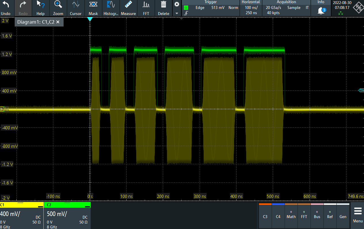
After uploading the command table as a vector to the correct node of the SHFSG+, we run the sequence, and start by measuring the following pulse sequences with the scope set to a time base of 700 ns/div.

From the results of this measurement, we can determine the control pulse
amplitudes needed for rotations of π or π/2. These amplitudes are
parametrized as QUBIT_PI_AMPLITUDE[qubit] and
QUBIT_PI_2_AMPLITUDE[qubit] in our LabOne Python API program,
respectively.
Ramsey Fringe Measurement
The Ramsey fringe measurement is also used to characterize our 2 qubits. The measurement starts by using a π/2 pulse to create an equal superposition of the excited and ground states. After waiting for a certain evolution time, we apply a second π/2 pulse, followed by the readout of the 2 qubits. Sweeping the evolution time between the two π/2 pulses gives us information about the coherence time of the qubit. Resonantly, which results in the exponential decay of the signal with respect to the coherence time, or we can drive the 2 qubits off-resonantly, which yields an oscillation of the signal at the detuning frequency.
This experiment starts by defining the different parameters needed for
the Ramsey measurement. We set the parameter
NUM_STEPS_RAMSEY_EXPERIMENT to 4, and add
NUM_AVERAGES_RAMSEY_EXPERIMENT = 1, RAMSEY_OFFSET_FREQUENCY=1e6 :
## define parameters
NUM_STEPS_RAMSEY_EXPERIMENT = 4
NUM_AVERAGES_RAMSEY_EXPERIMENT = 1
RAMSEY_OFFSET_FREQUENCY = 1e6
MAX_WAIT_TIME_TARGET = 1e-6
wait_time_steps_samples = int(round(MAX_WAIT_TIME_TARGET/(NUM_STEPS_RAMSEY_EXPERIMENT-1)*SAMPLING_RATE/16)*16)
QUBIT_PI_2_AMPLITUDE = [1,1]
Similarly to what we have seen before. We then define the waveforms and assigning them to the right index
After this, we define the variable evolution_time_samples which sets
the time separation between two π/2 pulses in the Ramsey experiment.
After receiving the trigger signal from the PQSC, the sequence executes
command table entry 0, which applies π/2 pulse to the qubit. A
playZero command follows the π/2 pulse to account for the evolution
time evolution_time_samples. Then we play a second π/2 pulse by
executing the command table entry 0 again. After applying a first Ramsey
sequence, we increment the time separation by +
wait_time_steps_samples for 4 times and we repeat this experiment one
time since NUM_AVERAGES_RAMSEY_EXPERIMENT = 1.
Additionally, we enable the digital modulation on both channels 1&2 of
the SHFSG+ and set the frequency of the oscillators to the sum of the
qubit frequency and the offset frequency, which is given by
RAMSEY_OFFSET_FREQUENCY=1e6. After configuring the outputs of both
channels, we finish by uploading the sequencer program to channels 1 & 2
of the SHFSG+.
for qubit in range(NUMBER_OF_QUBITS):
    seqc_program_sg[qubit]=f"""
    // Define a single waveform
    wave rabi_pulse=gauss({single_qubit_pulse_time_samples}, 1, {single_qubit_pulse_time_samples/2}, {QUBIT_SINGLE_GATE_TIME[qubit]*SAMPLING_RATE});

    // Assign a dual channel waveform to wave table entry
    assignWaveIndex(1,2,rabi_pulse, 1,2,rabi_pulse, 0);
    resetOscPhase();
    var i =0;
    // Trigger the scope
    setTrigger(1);
    setTrigger(0);
    repeat ({NUM_AVERAGES_RAMSEY_EXPERIMENT}) {{
        const evolution_time_samples = 0
        for (i = 0; i < {NUM_STEPS_RAMSEY_EXPERIMENT}; i++) {{
            waitZSyncTrigger(1);
            executeTableEntry(0);
            playZero(evolution_time_samples);
            executeTableEntry(0);
            waitWave();
            setTrigger(1);
            playZero(1024);
            waitWave();
            setTrigger(0);
            wait(5*{qubit_lifetime_samples});
            evolution_time_samples = evolution_time_samples + wait_time_steps_samples;


<table-caption identifier="Table">

        }}

<table-caption-end>

    }}
    """

    device.sgchannels[SGCHANNEL_NUMBER[qubit]].awg.modulation.enable(1)
    device.sgchannels[SGCHANNEL_NUMBER[qubit]].oscs[0].freq(QUBIT_DRIVE_FREQUENCY[qubit]+RAMSEY_OFFSET_FREQUENCY)

##upload programs
with device.set_transaction():
    device.sgchannels[SGCHANNEL_NUMBER[qubit]].awg.load_sequencer_program(seqc_program_sg[qubit])
In this case, the command table contains single entry and plays the dual-channel waveform referenced in the wave table at index 0. We specify the amplitude and the phase settings. The four amplitude settings of the command table are defined so that the output signal on both the channel 1&2 of the SHFSG+ plays a π/2 pulse. Then, we upload the command table as a vector to the correct node to the SHFSG+. After uploading the command table and the sequencer program, we run the sequence.
## create and upload command table
for qubit in range(NUMBER_OF_QUBITS):
    increment_value = MAX_DRIVE_STRENGTH[qubit]/NUM_STEPS_RABI_EXPERIMENT

    # Initialize command table
    ct_schema = device.sgchannels[sg_chan_index].awg.commandtable.load_validation_schema()
    ct = CommandTable(ct_schema)

    # Define pi/2 pulse
    ct.table[table_index].waveform.index = 0
    ct.table[table_index].amplitude00.value = 0.5*QUBIT_PI_2_AMPLITUDE[qubit]
    ct.table[table_index].amplitude01.value = -0.5*QUBIT_PI_2_AMPLITUDE[qubit]
    ct.table[table_index].amplitude10.value = 0.5*QUBIT_PI_2_AMPLITUDE[qubit]
    ct.table[table_index].amplitude11.value = 0.5*QUBIT_PI_2_AMPLITUDE[qubit]

    # Upload command table and enable sequencer
    device.sgchannels[SGCHANNEL_NUMBER[qubit]].awg.commandtable.upload_to_device(ct)
    device.sgchannels[SGCHANNEL_NUMBER[qubit]].awg.enable_sequencer(single = 1)
We show the expected result of the sequence in the Figure 5. As expected, we observe 5
pulse sequences of two consecutive π/2 pulses with increasing temporal
separation. The playZero command between two consecutive Gaussian
control pulses does not contribute to the memory use. Therefore, the
evolution time between the π/2 pulses can be extended to several seconds
without using waveform memory or increasing compilation and upload time.

Therefore, the evolution time between the π/2 pulses can be extended to several seconds without using waveform memory or increasing compilation and upload time.
Qubit Lifetime Measurement
In order to measure the lifetimes of the two qubits, we perform a T1 measurement on both qubits. The measurement starts after waiting for sufficiently long time \(\tau ( \tau>>T_1)\), so that the 2 qubits are in the ground state. Then, we excite both qubits by applying a π pulse to each qubit and wait for a variable amount of time before reading out the qubit state. The measured signal decays exponentially with respect to the delay time between control and readout pulses, with the time constant determined by the qubit’s lifetime.
We define the different parameters needed for the T1 measurement. We
start by setting the parameter NUM_STEPS_T1_EXPERIMENT to 5 and add
NUM_AVERAGES_T1_EXPERIMENT = 2**4 :
## define parameters
NUM_STEPS_T1_EXPERIMENT = 5
NUM_AVERAGES_T1_EXPERIMENT = 2**4
QUBIT_PI_AMPLITUDE = [2,2]
Similarly to what we have seen before, we define a variable time_ind,
which in this case sets the time separation between the control and
readout pulses. After receiving the trigger signal from the PQSC, we
execute the command table entry 0, which applies a π pulse to each
qubit. This is followed by a playZero command, which sets the time
separation between the control pulse and the readout signal.
The control channels are configured in the same way as in the Ramsey experiment. After configuring both channels of the SHFSG+, we finish by uploading the sequencer program to the AWG module for both SHFSG+ channels 1 & 2.
for qubit in range(NUMBER_OF_QUBITS):
    seqc_program_sg[qubit]=f"""
// Define a single waveform
wave rabi_pulse=gauss({single_qubit_pulse_time_samples}, 1, {single_qubit_pulse_time_samples/2}, {QUBIT_SINGLE_GATE_TIME[qubit]*SAMPLING_FREQUENCY});

// Assign a dual channel waveform to wave table entry
assignWaveIndex(1,2,rabi_pulse, 1,2,rabi_pulse, 0);
resetOscPhase();
//Trigger the scope
setTrigger(1);
setTrigger(0);
var time_ind = 0;
repeat ({NUM_AVERAGES_T1_EXPERIMENT}) {{
    for (time_ind = 0; time_ind < {NUM_STEPS_T1_EXPERIMENT}; time_ind++) {{
        waitZSyncTrigger(1);
        executeTableEntry(0);
        playZero({wait_time_steps_samples}*time_ind);
        waitWave();
        setTrigger(1);
        playZero(1024);
        waitWave();
        setTrigger(0);
        wait(5*{qubit_lifetime_samples});

    }}
}}
    """


##upload programs
with device.set_transaction():
    device.sgchannels[SGCHANNEL_NUMBER[qubit]].awg.load_sequencer_program(seqc_program_sg[qubit])
Here, the command table contains a single entry with an index 0. The chosen amplitude settings allow us to play a π pulse for both qubits. We upload the command table as a vector to the correct node of the SHFSG+. After uploading the command table and the sequencer program, we run the sequence.
## create and upload command table
for qubit in range(NUMBER_OF_QUBITS):
    increment_value = MAX_DRIVE_STRENGTH[qubit]/NUM_STEPS_RABI_EXPERIMENT

    # Initialize command table
    ct_schema = device.sgchannels[sg_chan_index].awg.commandtable.load_validation_schema()
    ct = CommandTable(ct_schema)

    # Define pi pulse
    ct.table[table_index].waveform.index = 0
    ct.table[table_index].amplitude00.value = 0.5*QUBIT_PI_AMPLITUDE[qubit]
    ct.table[table_index].amplitude01.value = -0.5*QUBIT_PI_AMPLITUDE[qubit]
    ct.table[table_index].amplitude10.value = 0.5*QUBIT_PI_AMPLITUDE[qubit]
    ct.table[table_index].amplitude11.value = 0.5*QUBIT_PI_AMPLITUDE[qubit]

    # Upload command table and enable sequencer
    device.sgchannels[SGCHANNEL_NUMBER[qubit]].awg.commandtable.upload_to_device(ct)
    device.sgchannels[SGCHANNEL_NUMBER[qubit]].awg.enable_sequencer(single = 1)
As expected, we observe 5 pulses with the π pulse amplitude, amplitude, with an increasing delay between the pi pulse and the readout pulse, as shown in the Figure 6.

Pulse-length Sweeps
Note
The length of any playZero and playHold commands must be a multiple
of 16 samples and a minimum of 16 samples.
In some scenarios, it may be necessary to sweep the duration of a pulse,
e.g. for a Rabi measurement in which the length of the pulse in samples
is swept instead of the amplitude. In such cases, the sequencer command
playHold enables efficient length sweeps to be performed. Just as
playZero instructs the sequencer to play 0 for a specified number of
samples without using waveform memory, the command playHold instructs
the sequencer to hold the last I and Q waveform values for a specified
number of samples without using waveform memory. The command playHold
can also hold the values of marker bits.
In the following sequence, we perform a length sweep of a common pulse
envelope: the duration of a flat-top Gaussian pulse is swept using the
playHold command:
seqc_str = """\
//Define constants
const AMP = 1;
const LENGTH = 32;
const WIDTH = LENGTH/8;
const LEN_STEP = 16;

//Waveform definition
wave wI = gauss(LENGTH, AMP, LENGTH/2, WIDTH);
wave wIr = cut(wI, 0, LENGTH/2 - 1); //rising edge of 16 samples
wave wIf = cut(wI, LENGTH/2, LENGTH - 1); //falling edge of 16 samples
wave m = marker(LENGTH/2, 1);
wave wIrm = wIr + m; //combine rising waveform and marker data
wave wIfm = wIf + m; //combine falling waveform and marker data

assignWaveIndex(1,2,wIrm,0);
assignWaveIndex(1,2,wIfm,1);

var t = 32;
repeat (6) {
  resetOscPhase();
  executeTableEntry(0);
  playHold(t);
  executeTableEntry(1);
  t += LEN_STEP;
}
"""

## Upload sequence
device.sgchannels[sg_chan_index].awg.load_sequencer_program(seqc_str)
After defining constants and assigning waveform indices, the sequence
plays a Gaussian rising edge of 16 samples (8 ns) using
executeTableEntry, followed by a playHold command. The length of the
playHold is swept from 32 to 128 samples (16 to 64 ns), in steps of 16
samples (8 ns) over the 6 iterations of the repeat loop. The playHold
is followed by the falling edge of the flat-top Gaussian pulse, also of
length 16 samples (8 ns).
We next define the corresponding command table, upload it, and enable the sequencer:
## Initialize command table
ct_schema = device.sgchannels[sg_chan_index].awg.commandtable.load_validation_schema()
ct = CommandTable(ct_schema)

## Waveform 1
ct.table[0].waveform.index = 0
## Waveform 2
ct.table[1].waveform.index = 1

## Upload command table
device.sgchannels[sg_chan_index].awg.commandtable.upload_to_device(ct)
## Enable sequencer
device.sgchannels[sg_chan_index].awg.enable_sequencer(single = single)
Observing the signal on the oscilloscope, we see that both the length of the waveform and the marker are swept as expected.