Pulse Generation and Acquisition with Timeline
This tutorial introduces the working principles of the Timeline module in the LabOne user interface when the AWG option of the instrument is installed. In this tutorial, the main aspects of the Timeline module, i.e. pulse generation and pulse acquisition are explained. It is intended for users who want to create and inspect pulse sequences in the Timeline module and capture the generated signals with the instrument's oscilloscope and demodulators.
Note
This tutorial is applicable to all SHFLI instruments with the SHFLI-AWG Arbitrary Waveform Generator option installed.
Preparation
Make sure the instrument is powered on and connected by Ethernet to your local area network (LAN), or by USB to your host computer. Start the LabOne User Interface as explained in Connecting to the Instrument. The LabOne Data Server and Web Server are automatically started and run in the background.
This tutorial uses the Signal Output 1 port to generate the pulses, and the Signal Input 1 port to measure them. Therefore, these two ports must be connected by an SMA cable in loop back.
Create a Pulse Sequence in the Timeline Editor
In the Setup space, bring the blocks for Signal Output 1 and Signal Input 1 to the canvas using the "+" menu on top of the screen. Adjust their signal settings like Range and Coupling according to Figure 1. Then, open the Timeline window from the bottom of the screen. The Timeline window includes 3 main areas: Editor, Viewer, and Settings. The Timeline editor allows you to build pulse sequences by placing waveform events on the timeline. Each event defines the channel, amplitude, duration, and timing of the generated waveform. The parameters of each event can be adjusted from the Settings area on the right.
Figure 1 shows a simple pulse sequence in the Timeline editor. The sequence consists of two pulse events with some delays in between and around that produce the output signal. The entire section is performed in a Single iteration.
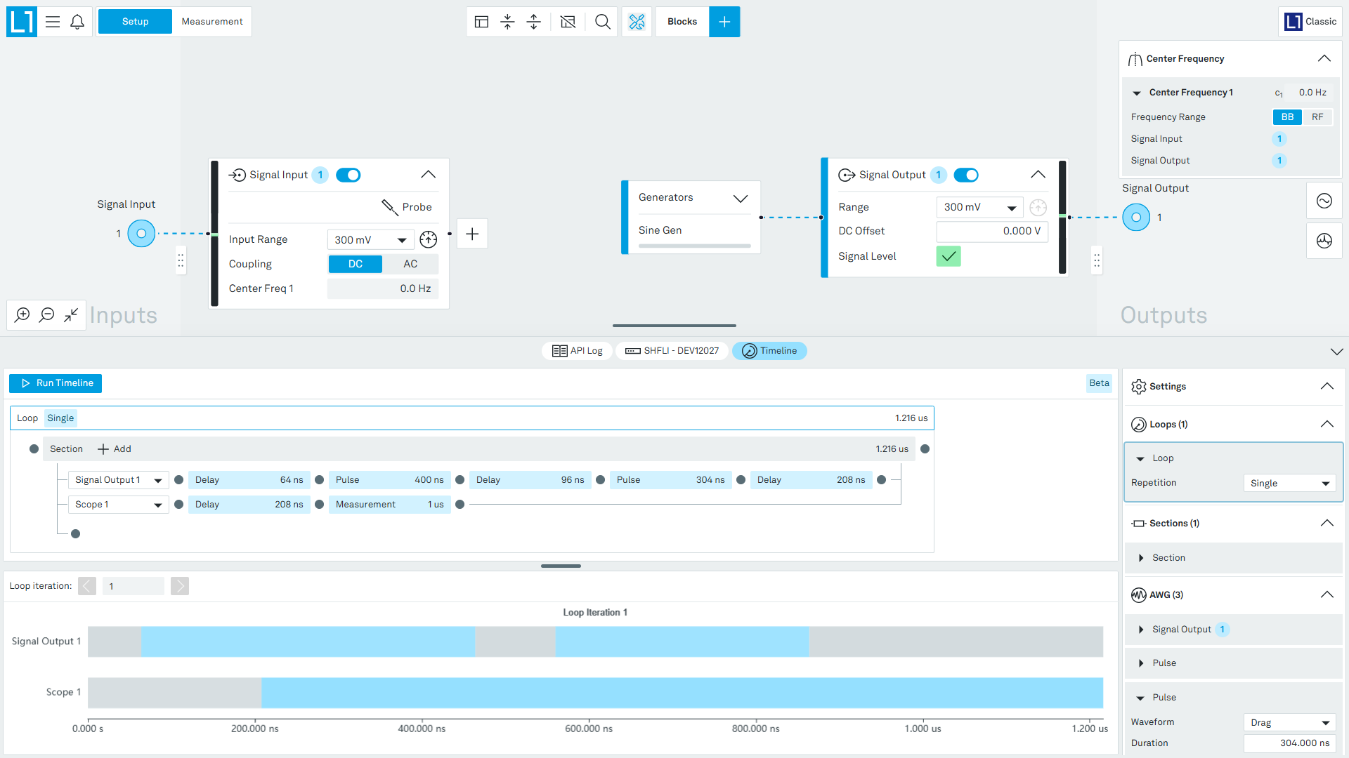
To build the sequence:
- Add Signal Output 1 under the Section in the Timeline editor.
- Add pulse and delay events using the editor controls.
- Adjust the pulse and delay parameters from the Settings area.
- Use the Timeline viewer to verify the event timing.
Once the sequence is configured, press the "Run Timeline" button to generate the corresponding signal on Signal Output 1. Note that the Signal Output and Input ports are in the base-band (BB) mode to generate and capture pulses without frequency up- and down-conversion.
Capture the Generated Pulses with the Scope
The Scope tool displays the received waveform on the Signal Input 1 port. It is useful for verifying the pulse shape, amplitude, and timing. Add the Scope to the Timeline editor as a measurement line with time-adjusted delay and measurement boxes. By opening the Scope tool in the Measurement space, and running the Timeline, the captured pulses can be displayed as a trace or an image as seen in Figure 2. The signal trace corresponds to the waveform defined in the Timeline editor which includes a Gaussian pulse followed by a Drag pulse.
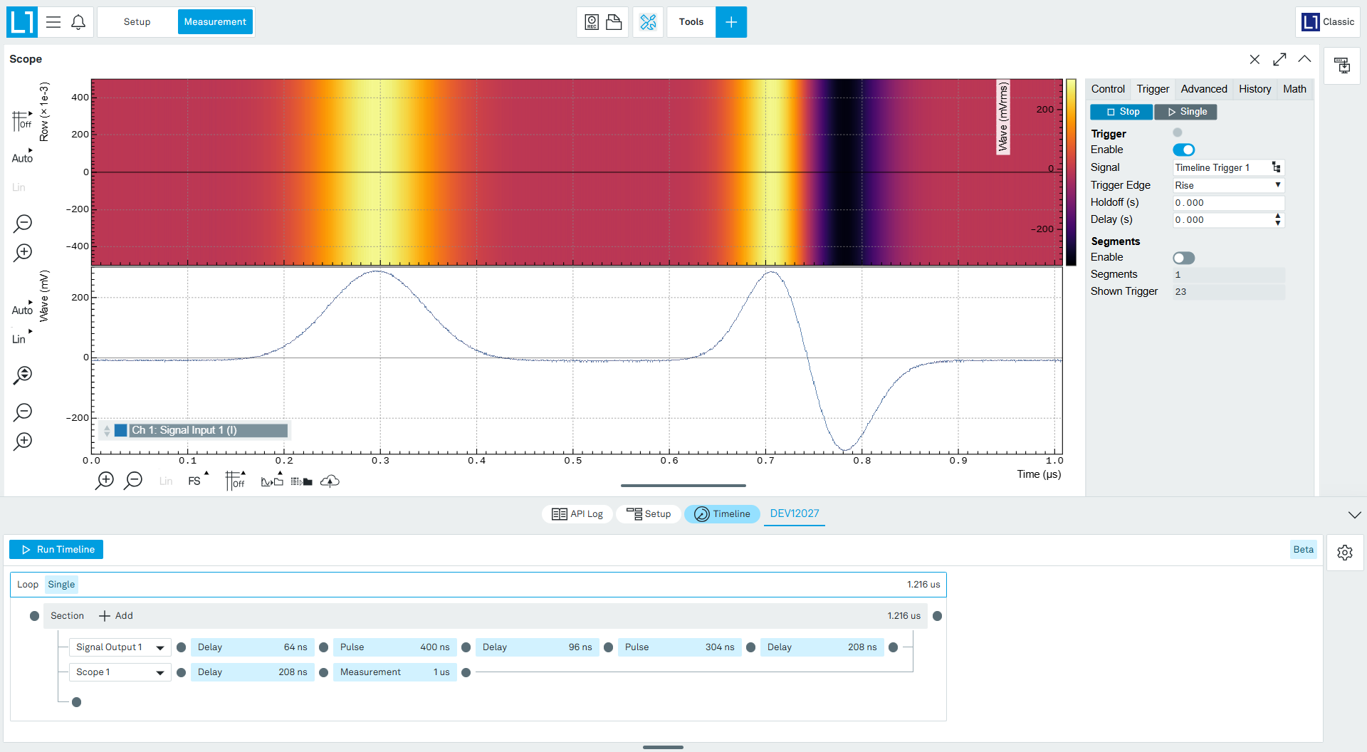
If the waveform does not appear as expected, check the event parameters in the Timeline editor as well as the Scope settings. Note that the same Timeline module can be accessed from the Setup and Measurement spaces.
Apply Amplitude Modulation
The SHFLI Lock-in Amplifier offers two modes of operation when it comes to signal frequency, i.e., base-band (BB) and radio-frequency (RF). In the RF mode, the waveform generated by the Timeline module will be up-converted to the center frequency. Therefore, the signal leaving the output port and arriving at the input port includes modulation at microwave frequency.
Regardless of the RF and BB frequency range, the Timeline module can apply amplitude modulation to the generated waveform. This feature enables the envelope modulation using a sine generator linked to one of the instrument's numeric oscillators. In RF, this means shifting the modulation carrier around the center frequency by the numeric oscillator's frequency.
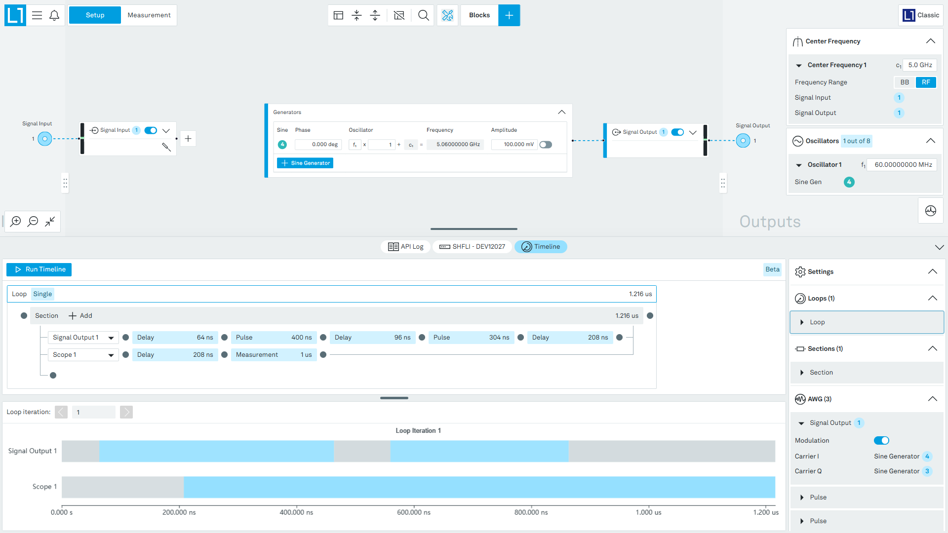
To apply the modulation, enable the corresponding feature in the Timeline settings as seen in Figure 3. The selection of oscillator, phase, and harmonic can be done in the Generators block attached to the Signal Output block.
In case of RF mode, the outcome frequency of modulation carrier is the sum of the center frequency and numeric oscillator. For instance, the carrier frequency of the generated signal in Figure 3 is 5.0 GHz + 60 MHz = 5.06 GHz as displayed in the Generators block.
When modulation is enabled, the generated signal follows the defined envelope shape but oscillating according to the modulation frequency of the Sine Generator. Figure 4 shows the modulated waveform captured by the Scope tool.
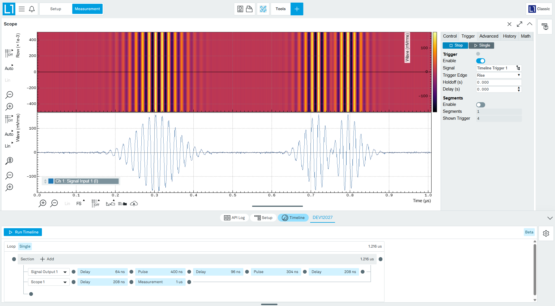
By modifying the numeric oscillator's frequency, the modulation carrier can be set anywhere within the instrument's frequency range.
Demodulate the Received Signal
To obtain the envelope of the modulated pulses, add a demodulator to the Signal Input block as seen in Figure 5. The demodulator uses the same oscillator as the modulation carrier created by the Sine Generator. Moreover, the acquisition window is set by adding a Measurement line to the Timeline editor which is assigned to the corresponding Demodulator with properly adjusted Delay and Measurement boxes.
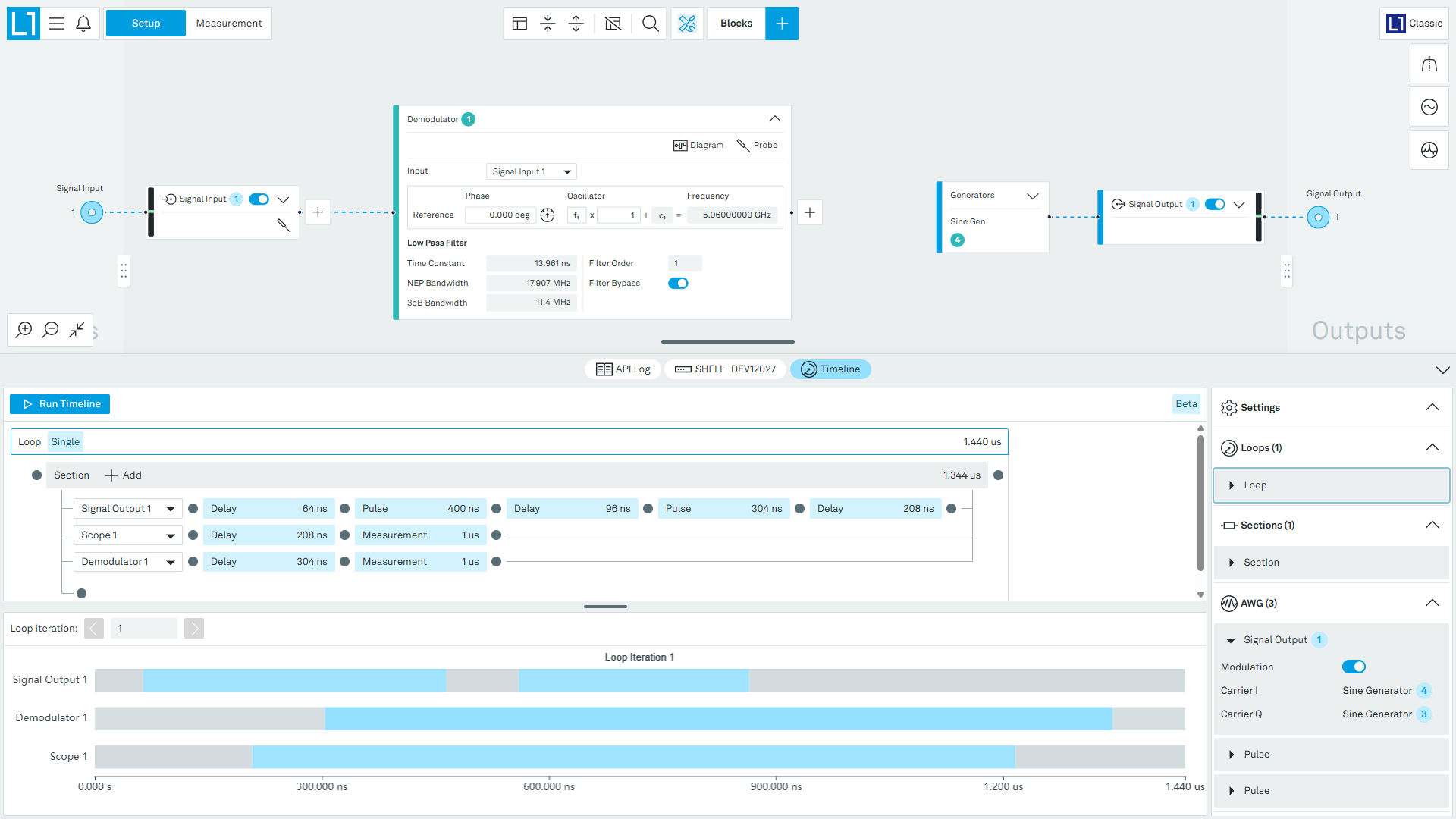
Use the Timeline viewer to verify that the sequence of events are aligned with the expected timing of pulse generation and acquisition.
In the RF mode, there is down-conversion to the intermediate band in the Signal Input port before demodulating the signal by the numeric oscillator. As a result, the demodulation frequency is obtained from the sum of the center frequency and numeric oscillator. In Figure 5, the final demodulation frequency is 5.0 GHz + 60 MHz = 5.06 GHz as displayed in the Demodulator block.
Inspect the Waveform in the Timeline DAQ
The Timeline DAQ tool in the Measurement space provides time-domain and frequency-domain monitoring of the acquired signal after demodulation. It is useful for checking the temporal and spectral content of the played pulse sequence, and confirming that the output matches the intended waveform.
Figure 6 shows the temporal (left) and spectral (right) content of the demodulated pulses captured by the Timeline DAQ tool. The time-domain traces are the quadrature components of the demodulated signal; while the frequency-domain trace displays its two-sided spectrum.
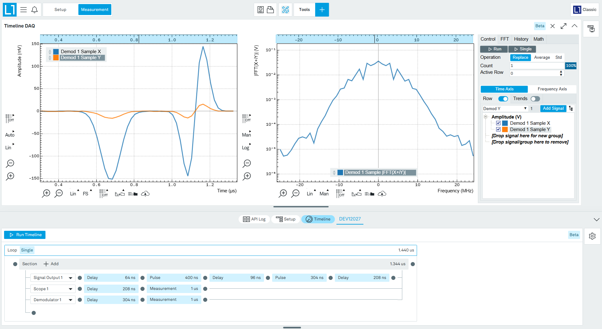
Note that different signal components like amplitude, phase, and their spectrum can be added to the list of signals captured by the Timeline DAQ tool. Regardless of BB or RF selection, the outcome of demodulation is in the base-band frequency range. This is achieved, in the RF mode, first by down-conversion of the received signal and then demodulation of the down-converted result.