Simple Loop
This tutorial is for users with little or no prior experience with Zurich Instruments lock-in amplifiers. Using a basic measurement setup, it introduces the fundamental working principles of the VHFLI and the LabOne user interface in a step-by-step approach.
Note
This tutorial is applicable to all VHFLI instruments. No additional option is required.
Preparation
In this tutorial, you will generate a single-ended signal with the VHFLI and measure it with the same instrument using an internal reference. This is done by connecting Signal Output +V to Signal Input +V of one of the two channels with a short BNC cable (ideally < 30 cm). We recommend using one of the 2 BNC cables included with the VHFLI. It is also possible to connect the generated signal to an oscilloscope by using a T-connector and an additional BNC cable. Figure 1 displays a sketch of the hardware setup.
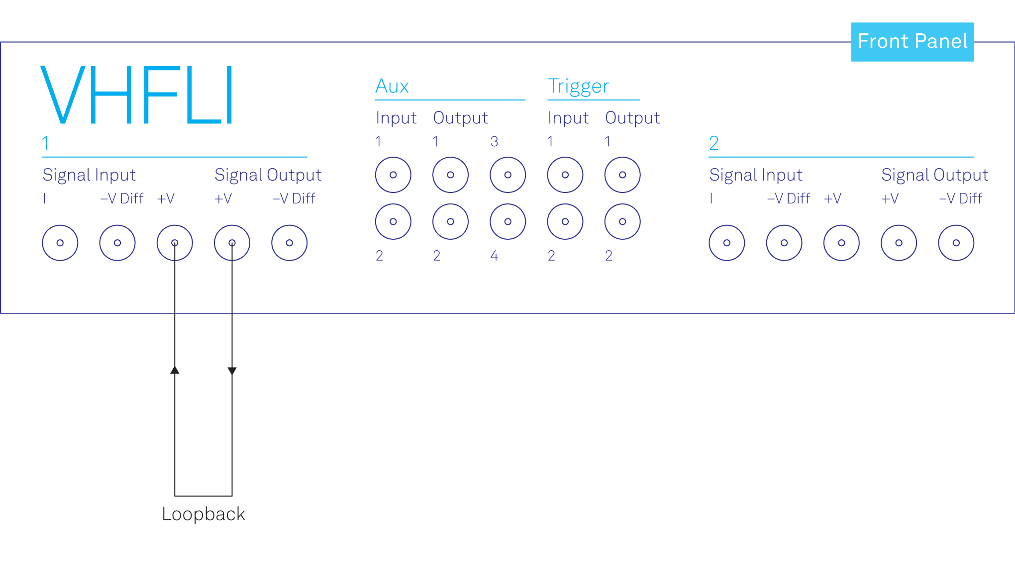
Make sure the VHFLI is powered on and successfully connected to the controlling PC (see Getting Started for details). The tutorial can be started with the default instrument configuration and the default user interface settings. Once LabOne is started, the Setup Workspace is shown on the screen. In case some blocks are already present on the canvas, you can remove them by clicking on the “Delete all blocks” button in the top center of the Setup workspace.
Generate and visualize the Test Signal
Note
The following steps use channel 1. If you are using channel 2, replace all instances of Signal Input 1 and Signal Output 1 with Signal Input 2 and Signal Output 2.
In the Setup workspace, click on the Blocks button (the "+" symbol in the top bar) to open the dropdown menu. Select Signal Output 1 from the submenu as shown in Figure 2. This will add the Signal Output 1 block to the canvas, allowing you to generate the test signal.
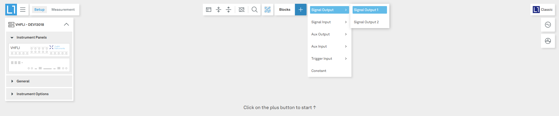
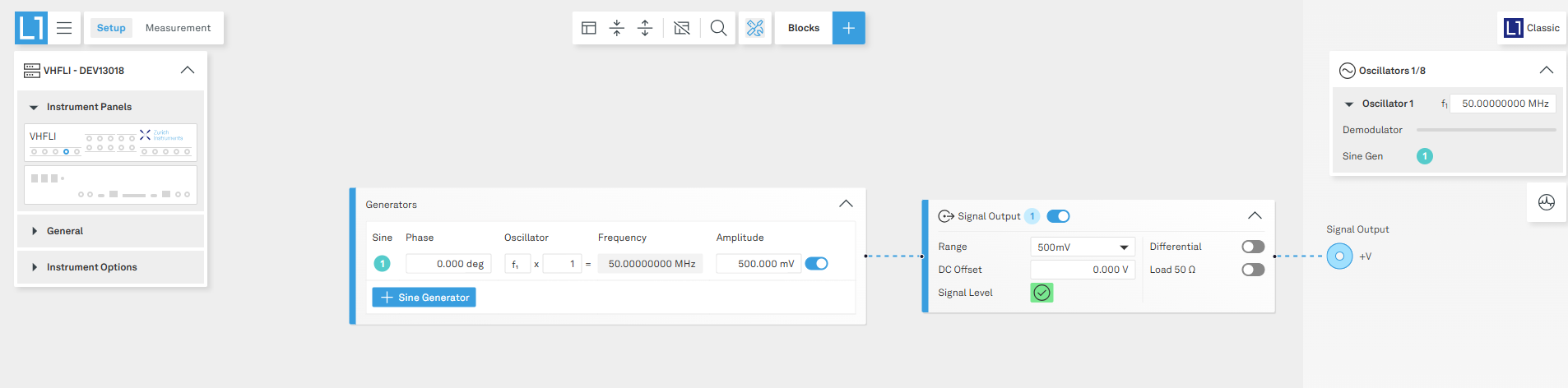
After adding the block, configure the Signal Output 1 block as follows:
- Enable the sine generator.
- Set the frequency to 50 MHz in the Oscillators panel on the right.
- Set the Range to 500 mV.
- Enable the On/Off toggle switch at the top of the block to activate the output.
The oscillator frequency settings will appear on the right-side Oscillators panel; see Figure 3.
To begin the demodulation process, add the Voltage Input 1 block to the canvas by clicking on the “+” button in the top bar and selecting Signal Input 1. Once the block is on the canvas, set the input range to 1.0 V and ensure the AC, 50 Ω, Diff, and Float options are disabled; see Figure 4.
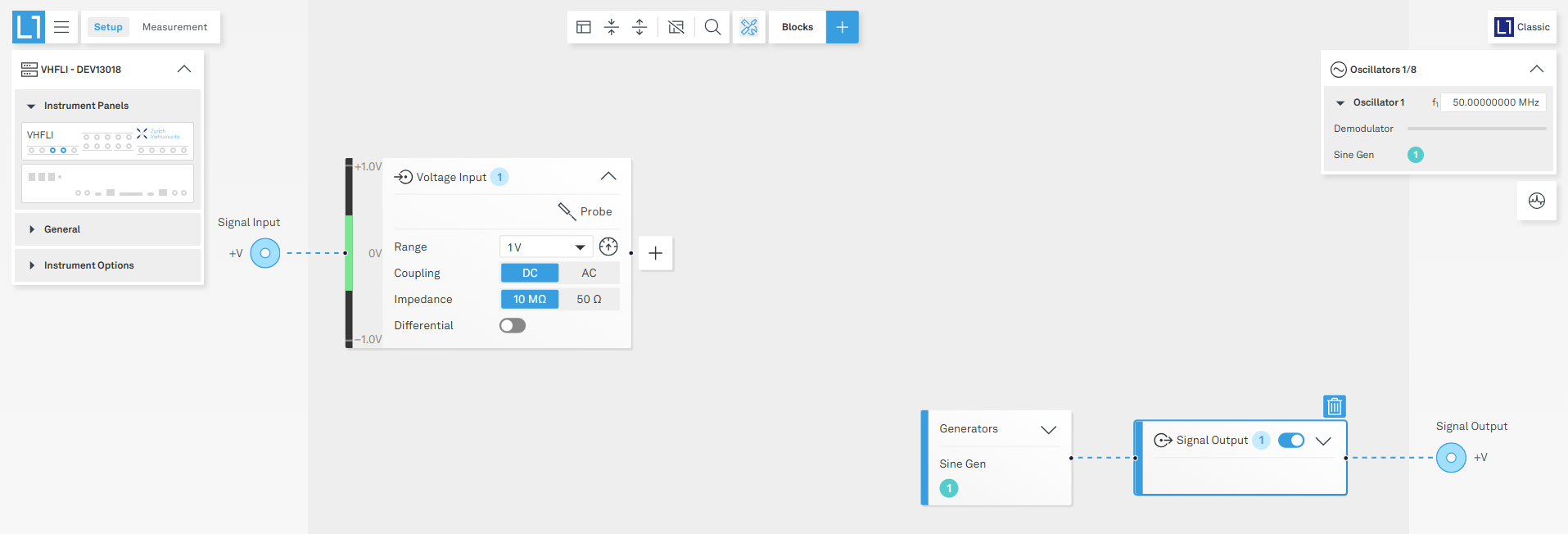
The range setting ensures that the resolution of the input analog-to-digital converter is used efficiently without clipping the signal to optimize the dynamic range.
The incoming signal can now be observed over time using the Scope tool; click the probe icon in the Voltage Input block, as shown in the following figure.
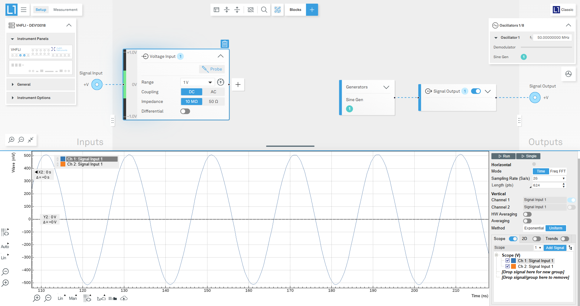
Demodulate the Test Signal
You are now ready to demodulate the input signal and measure its amplitude and phase.
- Add a Demodulator block by clicking the “+” on the right-hand side of the Voltage Input block. This connects it to the signal input.
- On the Demodulator block, set the low-pass filter to a 3 dB bandwidth of 1 kHz with a 4th order filter.
Choosing a low-pass filter value is always a tradeoff between noise rejection and measurement speed. The demodulator uses the same oscillator set up in the signal generation steps. Optionally, the measurement result can be routed to an Auxiliary Output by adding the corresponding connection on the Demodulator block.
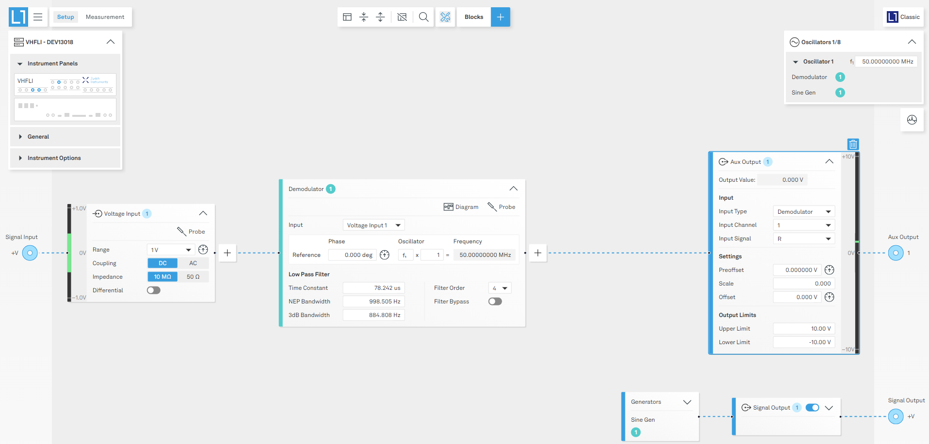
Plot the measurement results
To view and analyze your measurement results, switch to the Measurement workspace by clicking on the Measurement tab in the top-left corner of the interface. In this workspace, you have access to a variety of powerful visualization tools. For example, you can use the Plotter to display the time trace of your demodulated data, allowing you to observe amplitude variations directly over time. Alternatively, you can select the Spectrum Analyzer to gain insights into the frequency domain representation of your measured signals. These and all the other analysis tools are available by clicking on the “+” button in the top-center part of the interface.
On the right-side panel, make sure to enable the Data Transfer toggle for the relevant demodulator channel to ensure your data is sent to the visualization tools. It is important to set a suitable Data Rate for data transfer. This rate should be matched to the low-pass filter setting of your demodulator to achieve optimal sampling; note that you can click the button next to the data rate setting to let the software automatically adjust the data rate for you. Configuring these settings appropriately ensures you capture all relevant measurement information without unnecessarily high data rates or insufficient sampling.
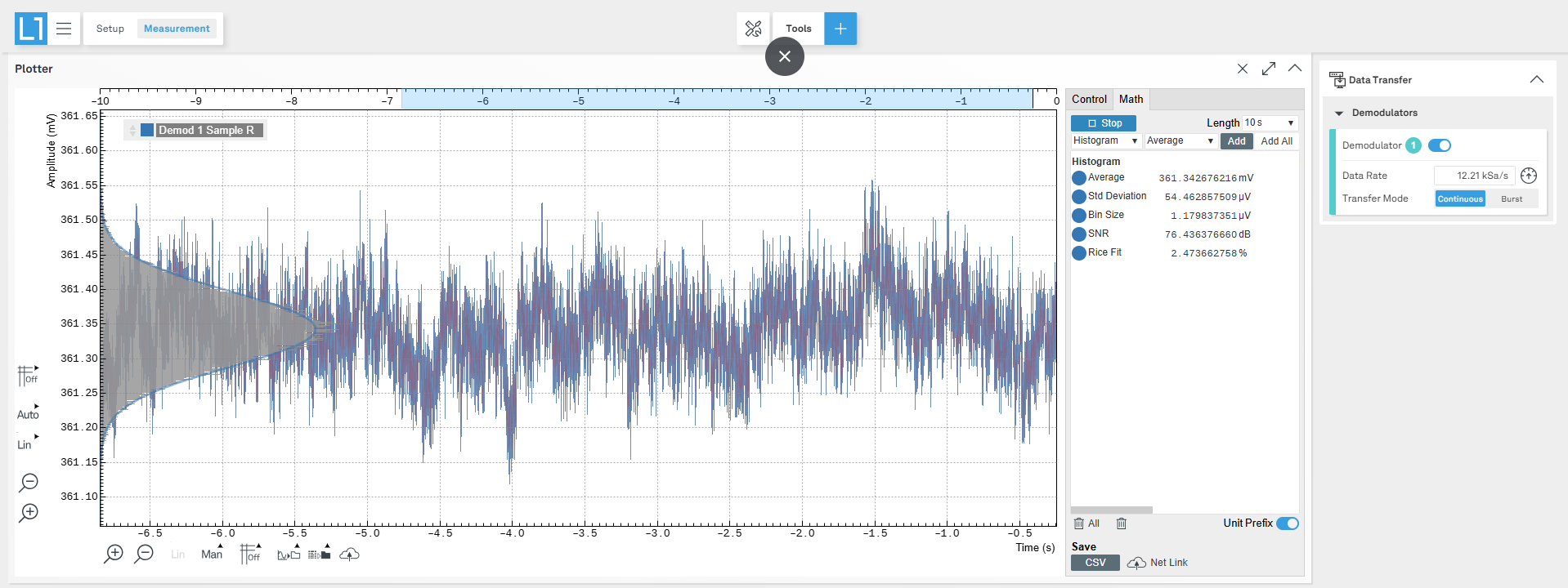
The average value of the measured signal in the plotter is about 351 mV, as expected from a 500 mV peak-to-peak sinusoidal input, taking into account the typical √2 factor stemming from the demodulation process. Additional insights, as well as statistics on the signal, can be gained through the Math sub-tab of the Plotter. See Figure 8 for an example of the Measurement workspace.
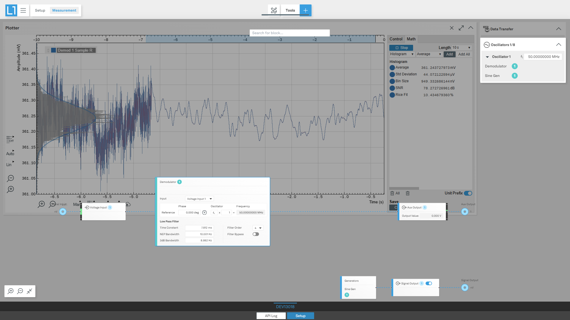
To adjust parameters in real time (e.g. the low-pass filter time constant), overlay the setup diagram in the measurement workspace by clicking “Setup” in the lower part of the screen (see Figure 8). Changes are reflected instantly in the visualization tool. In the example shown, the low-pass filter bandwidth is reduced to about 10 Hz, and the effect on the demodulated data is visible in the plotter. Alternatively, you can add the setup as a standalone block in the measurement workspace by clicking on the “+” button and selecting “Setup”.