Phase-locked Loop¶

This tutorial explains how to track the resonance frequency of a resonator over time using a phase-locked loop (PLL). You will first characterize the resonator with a frequency sweep and a curve fit, then close a feedback loop that holds the measured phase constant by steering the oscillator frequency. The frequency the loop settles on is the resonance frequency, and following it over time is a sensitive measure of anything that shifts the resonance, such as temperature, mass loading or stress.

Note

This tutorial is applicable to all VHFLI instruments with the VHF-PID Multi PID/PLL Controller Option installed. The instrument used for the screenshots also has the VHF-MD Multi-demodulator option installed, so some panels may show more channels than yours.

Preparation¶

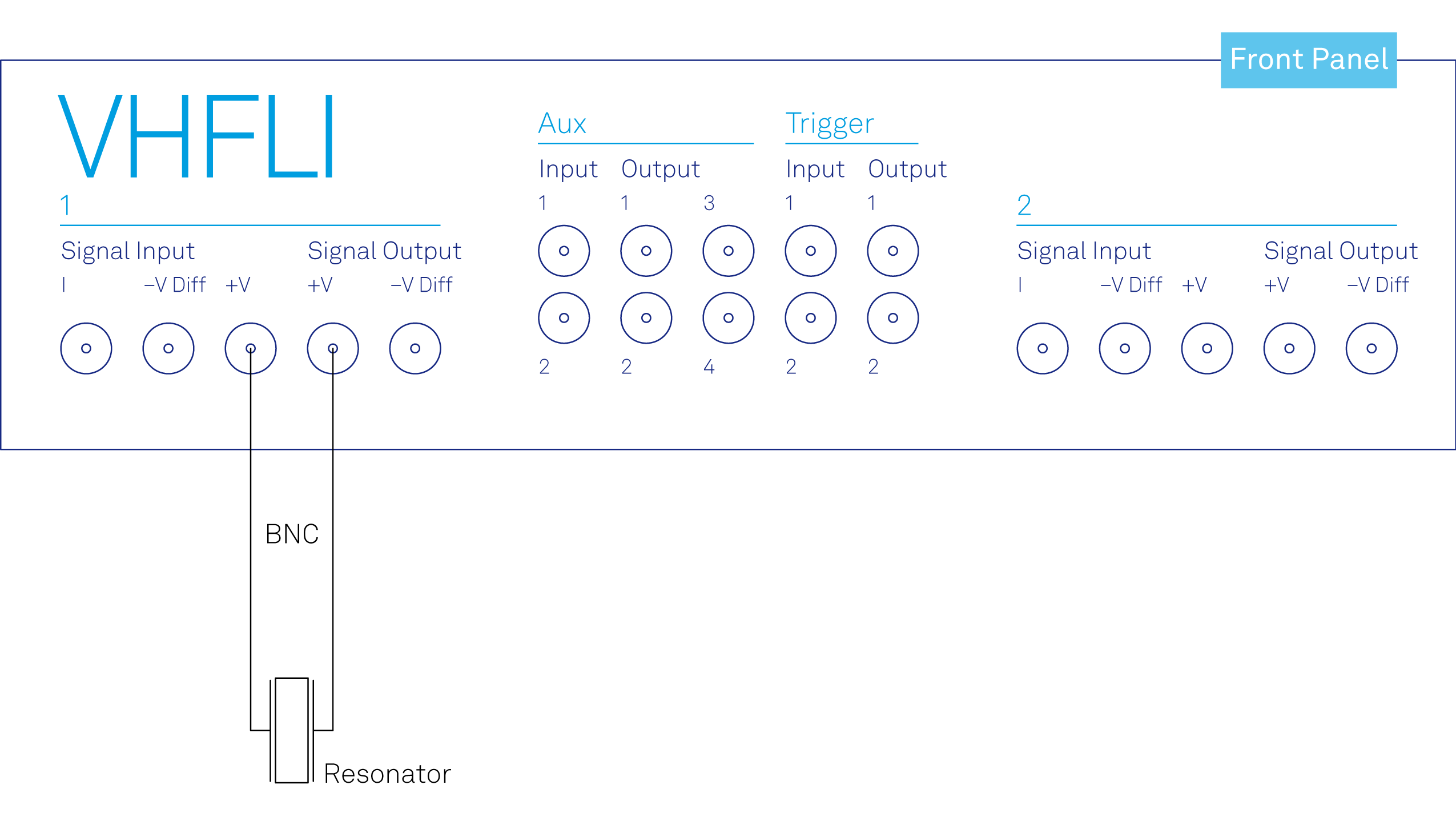
To follow this tutorial you need a resonator, ideally a quartz crystal, connected between Signal Output 1 +V and Signal Input 1 +V, as shown in Figure 1. The example uses a crystal with a resonance near 1.84 MHz. The PLL operates from 1 Hz to 50 MHz, or to 200 MHz with the VHF-F200M option, so choose a resonator whose resonance falls inside that range.

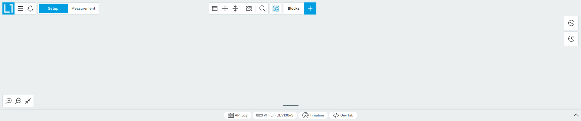
Figure 1: Setup for the phase-locked loop tutorial. The resonator is connected between Signal Output 1 and Signal Input 1.

Make sure the VHFLI is powered on and successfully connected to the controlling PC (see Getting Started for details). The tutorial can be started with the default instrument configuration and the default user interface settings. Once LabOne is started, the Setup workspace is shown on the screen. If blocks are already present on the canvas, remove them with the Delete all blocks button at the top center of the workspace (Figure 2).

Figure 2: The empty Setup workspace. Blocks are added from the plus button in the top bar.

Build the Signal Chain¶

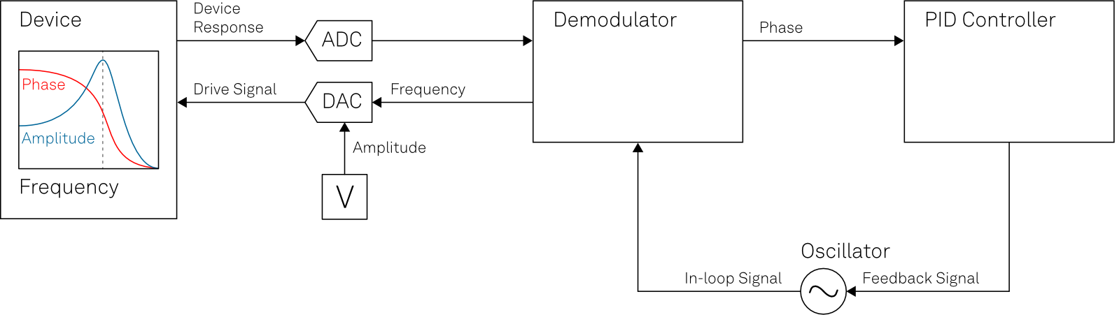
The measurement needs four things on the canvas: a sine generator to drive the resonator, a signal input to receive what comes back, a demodulator to measure the amplitude and phase of the transmitted signal, and a PID controller to control the frequency of the sine generator, closing the loop.

Figure 3 shows how these elements work together. The oscillator sets the frequency of the drive signal, which reaches the device through the DAC, and the sine generator sets its amplitude. The response of the device returns through the signal input and the ADC to the demodulator, which measures the amplitude and the phase at the drive frequency. The PID controller compares that phase with a setpoint and feeds a correction back to the oscillator, so the drive frequency follows the resonance as it shifts.

Figure 3: Block diagram of the phase-locked loop. The demodulator measures the phase of the device response, and the PID controller steers the oscillator frequency to hold that phase constant.

You will build the first three elements here, then add the PID controller in the next section, where it also gives you the Advisor used to characterize the resonance.

In the Setup workspace, click the Blocks button (the plus symbol in the top bar) and select Signal Output 1, as shown in Figure 4.

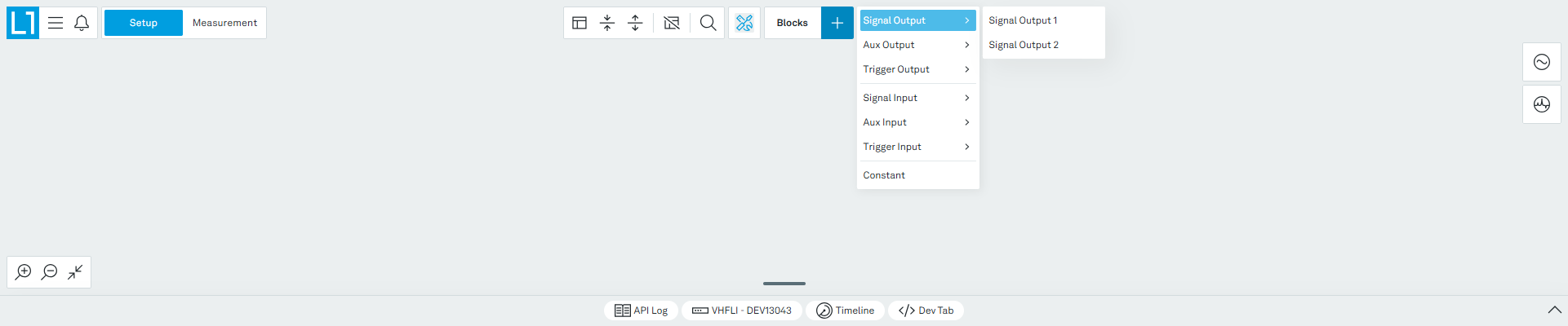
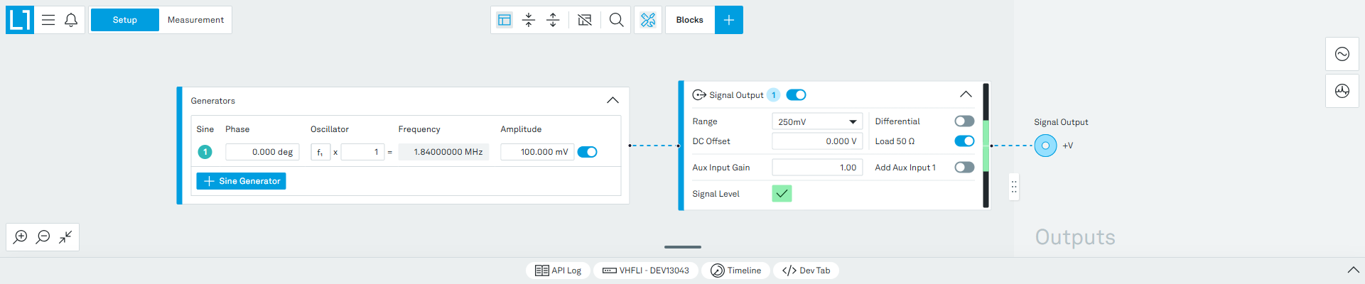
Figure 4: Adding the Signal Output 1 block from the Blocks menu.

Adding Signal Output 1 also places a Generators block on the canvas, attached to its input. The Generators block cannot be added on its own, as it always belongs to a signal output. Configure the two blocks as follows:

In the Generators block, click + Sine Generator to add a sine generator, and set its Amplitude to 100 mV.
Set the frequency in the Oscillators panel on the right-hand side. Enter a first estimate of the resonance. Here we use 1.84 MHz. The exact value is measured later.
In the Signal Output block, set the Range to 250 mV and enable Load 50 Ω.
Enable the sine generator with the toggle in the Generators block, and switch the output on with the toggle in the Signal Output block header.

The drive amplitude is set in the Generators block, while the output range is set in the Signal Output block. Figure 5 shows both blocks together with the Oscillators panel. The green check mark next to Signal Level confirms that the requested amplitude fits inside the selected range.

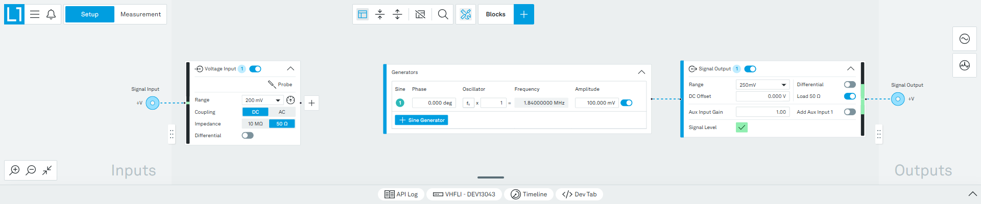
Figure 5: The Generators block with one sine generator at 100 mV, the Signal Output block set to the 250 mV range with Load 50 Ω enabled, and the Oscillators panel where the frequency is set.

Next, add the input. Click the plus button in the top bar again and select Signal Input 1. The block appears on the canvas labeled Voltage Input 1. Set Coupling to DC, Impedance to 50 Ω, and leave Differential switched off (Figure 6). The 50 Ω termination matches the cable and gives the resonator a defined load, which is what makes the phase response behave as described below.

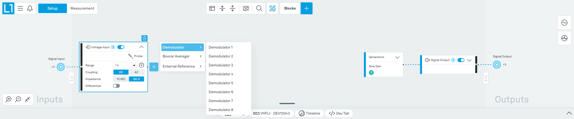
Figure 6: The Voltage Input block with 50 Ω input impedance, DC coupling and single-ended input.

To measure the transmitted signal, click the plus on the right edge of the Voltage Input block and select Demodulator, as shown in Figure 7.

Figure 7: Adding a Demodulator from the plus button on the right edge of the Voltage Input block.

Set the demodulator low-pass filter to a 3 dB bandwidth of about 93 Hz with a 3rd order filter, corresponding to a time constant of 874 µs. A bandwidth comparable to the linewidth of the resonance is a reasonable starting point.

The completed chain is shown in Figure 8. In the Oscillators panel on the right, both Sine Gen 1 and Demodulator 1 are listed under Oscillator 1. The same oscillator generates the drive and demodulates the response, so the phase reported by the demodulator is the phase shift of the resonator itself.

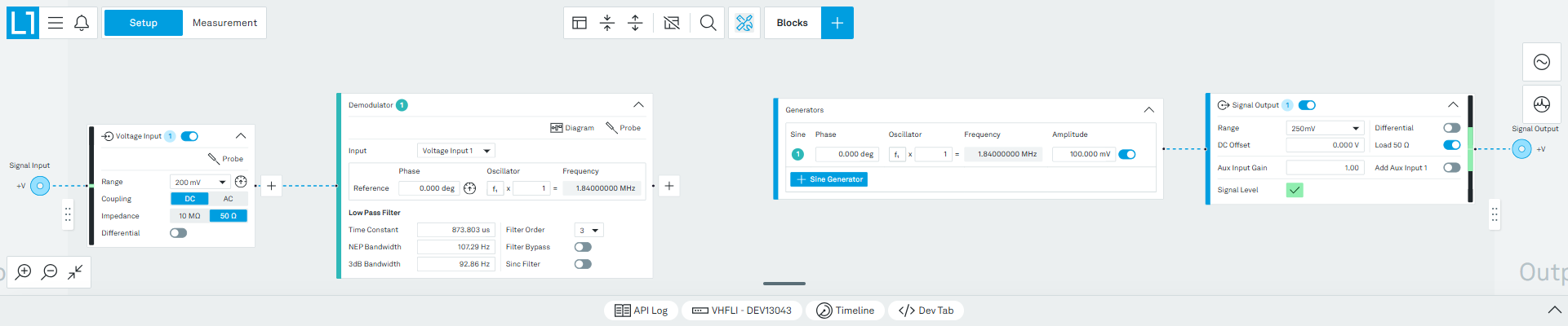
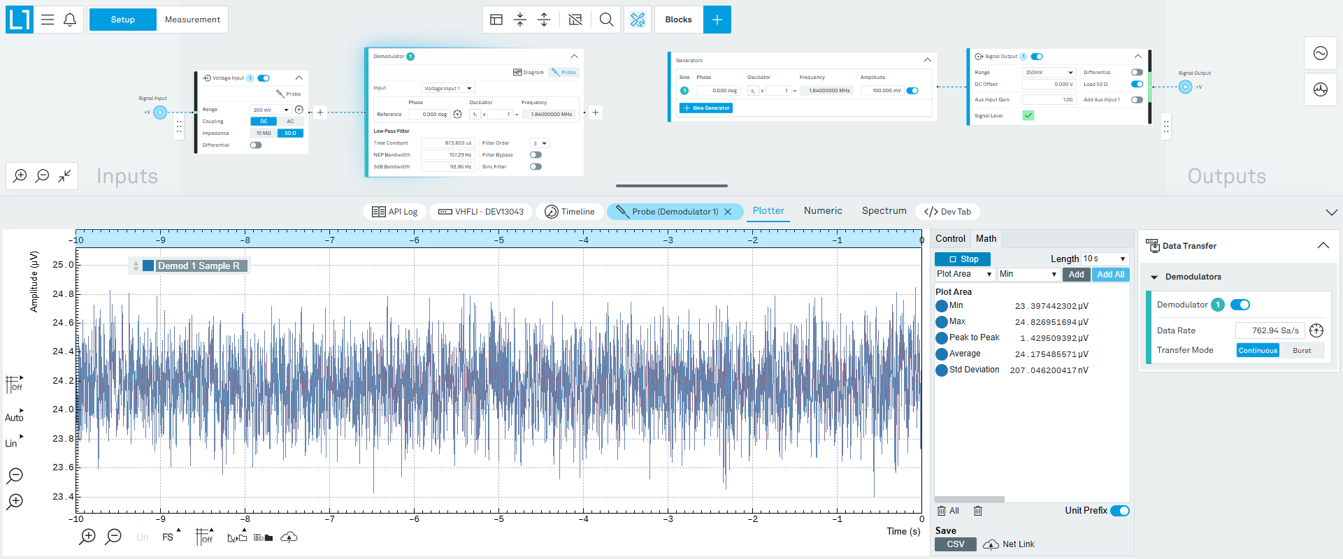
Figure 8: The complete signal chain. The Oscillators panel shows that the sine generator and the demodulator share Oscillator 1.

You can inspect the transmitted signal at any point without leaving the Setup workspace: click the Probe icon on the Demodulator block to open a plotter on its signals directly, as in Figure 9.

Figure 9: A probe plotter opened from the Demodulator block, showing the transmitted signal.

Characterize the Resonance and Configure the PLL¶

Now that the resonator is driven and measured, the drift of its resonance can be tracked by locking to the phase at resonance, hence the name phase-locked loop. The VHFLI has several PID controllers with PLL capability; this tutorial uses PID Controller 1.

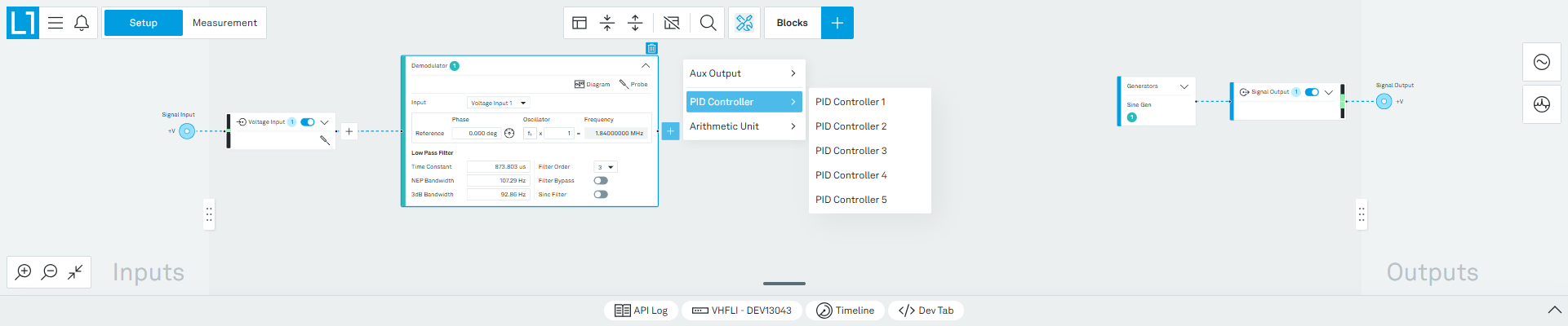
Click the plus on the right edge of the Demodulator 1 block and select PID Controller, as shown in Figure 10. Adding the controller this way sets its input Source to the demodulator automatically.

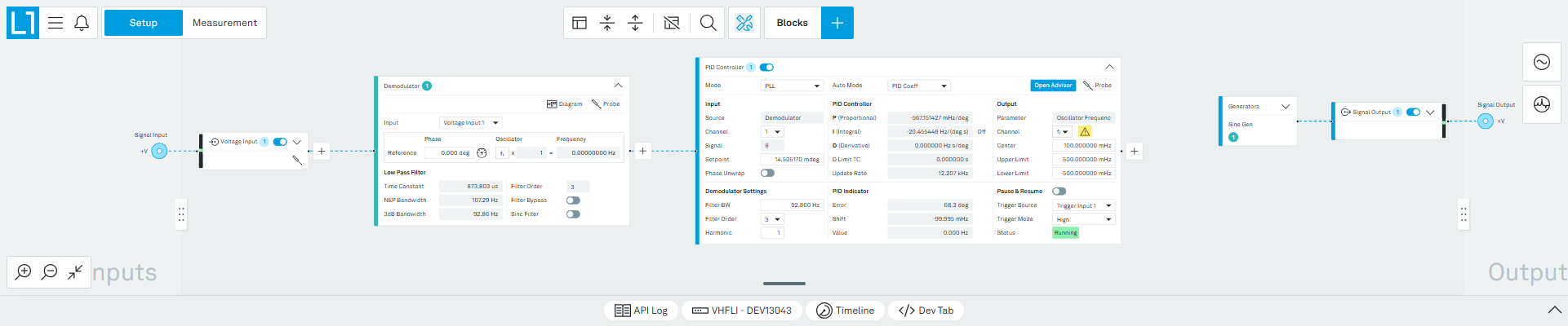
Figure 10: Adding a PID Controller from the plus button on the right edge of the Demodulator block.

In the block header, set Mode to PLL and Auto Mode to PID Coeff (Figure 11). Selecting PLL also sets the input Signal to θ. The available Auto Mode settings are Off, PID Coeff, Coeff + BW (low) and Coeff + BW (high).

Figure 11: The PID Controller block header with Mode set to PLL and Auto Mode set to PID Coeff.

Click Open Advisor in the PID Controller block header. A PID advisor panel opens at the bottom of the screen (Figure 12), containing a Guide with the steps to follow, the Advisor itself, and its own Sweeper and Plotter. The whole characterization is done here, so there is no need to switch to the Measurement workspace. If you only want to sweep a signal and do not need a PID or PLL, a standalone Sweeper is available in the Measurement workspace instead.

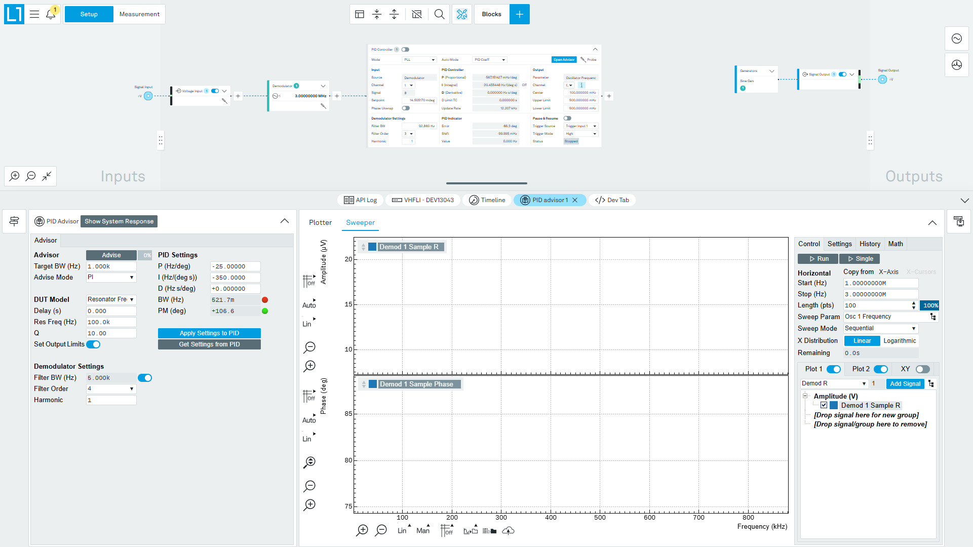
Figure 12: The PID advisor panel docked at the bottom of the screen, with the Guide, the Advisor, and its own Sweeper and Plotter.

First find the resonance with the Advisor's Sweeper. Configure its Control sub-tab as shown in Figure 13:

Set Sweep Param to Osc 1 Frequency.
Set Start to 1 MHz and Stop to 3 MHz, with a Length of 100 points, Sweep Mode Sequential and a Linear X Distribution.
Enable Plot 1 and Plot 2, then add Demod R to one plot and Demod Θ to the other using the signal selector and the Add Signal button.
Click Run to sweep repeatedly, or Single for one pass.

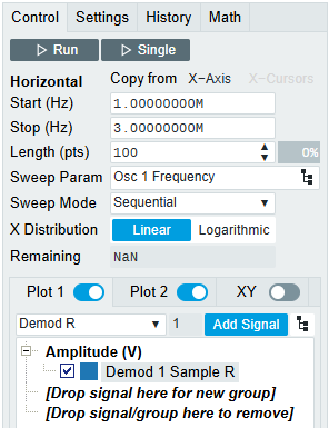
Figure 13: The Sweeper Control sub-tab in the PID advisor, configured for a coarse frequency sweep from 1 MHz to 3 MHz.

The result of the coarse sweep is shown in Figure 14. Several resonances are visible, which is normal for a quartz crystal. This tutorial follows the lowest one, near 1.84 MHz, but the method works equally well on any of them.

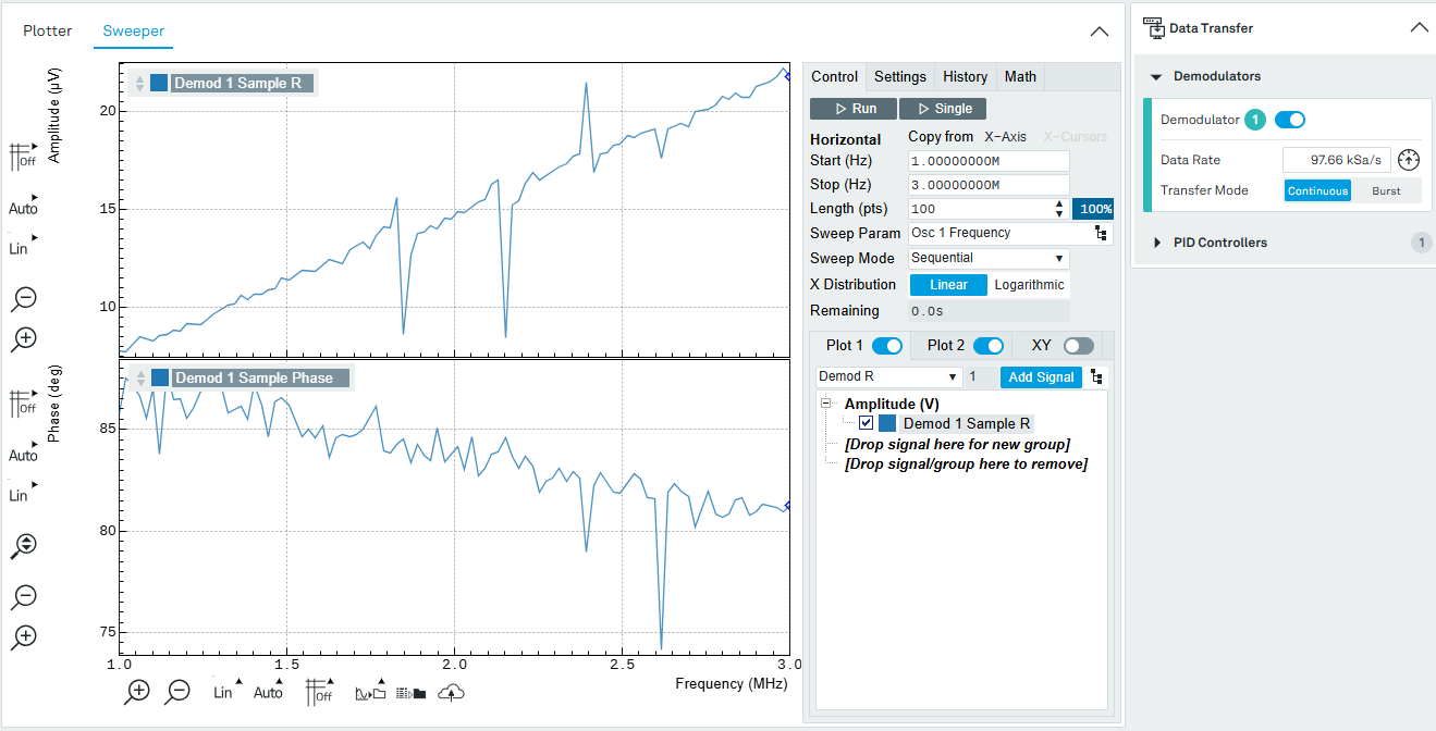
Figure 14: Coarse sweep from 1 MHz to 3 MHz. The crystal shows several resonances; this tutorial follows the one near 1.84 MHz.

To resolve the resonance, narrow the sweep range around it. There are two ways to do this:

Place the two X cursors on either side of the peak and click Copy from → X-Cursors.
Zoom in on the plot around the peak and click Copy from → X-Axis.

Either method transfers the range into the Start and Stop fields. Sweeping again over the narrower range gives a finer frequency resolution even with the same number of points. Repeat until the resonance fills the plot.

The resonance parameters can now be extracted with the Resonance fit in the Math sub-tab:

Select Resonance from the left drop-down menu.
Click Add All to add all of the fit results at once. Alternatively, select an individual result in the right drop-down menu and click Add to add them one at a time.

The tool performs a least-squares fit to the response of an LCR circuit. For a large quality factor this is a Lorentzian for the amplitude trace and an inverse tangent for the phase trace. It reports the quality factor Q, the 3 dB bandwidth, the center frequency, the amplitude or the phase at the center, and the fit error.

Perform the fit twice, once with the amplitude trace active and once with the phase trace, as the two are fitted independently. Both sets of results are then listed together in the Math sub-tab, as in Figure 15.

For the crystal measured here the amplitude fit gives

Q = 16.834 × 10³, bandwidth 109.470 Hz, frequency 1.8428 MHz, amplitude 536.4 μV, fit error 2.37 %

and the phase fit gives

Q = 16.490 × 10³, bandwidth 111.750 Hz, frequency 1.8428 MHz, phase −4.9538°, fit error 0.31 %

The two agree to about 3 % in Q and to a few Hz in center frequency, which indicates the resonator is well described by the LCR model. Where the two disagree, often because of capacitive coupling between the leads, the phase fit is usually the more reliable of the two. Here it also has by far the smaller fit error.

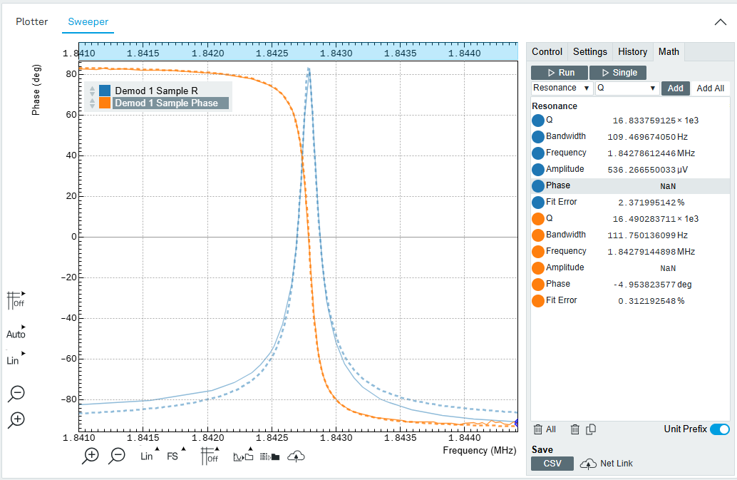
Figure 15: Resonance fit results in the Math sub-tab. The upper set of values is the fit to the amplitude trace, the lower set the fit to the phase trace.

The phase follows the response typical of a resonator on a 50 Ω input, approaching +90° well below the resonance and −90° well above it, and passing close to 0° at the resonance itself. The exact value at the resonance, −4.9538° from the phase fit, is the quantity the feedback loop will hold constant.

With the resonance characterized, fill in the PID Controller Input and Output fields from the fit:

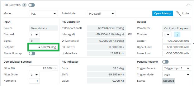
Under Input, enter the phase measured at the resonance (in our case, −4.9538 deg) as the Setpoint.
Under Output, set Parameter to Oscillator Frequency and Channel to f₁, the same oscillator that drives the resonator.
Set Center to the fitted resonance frequency. Here we entered 1.8428 MHz.
Set the initial Upper and Lower Limit. Here we use the default +500 mHz and −500 mHz.

The limits define how far the loop may move the frequency away from the center. They must be narrow enough that the phase of the device follows a monotonic curve with a single crossing at the setpoint, otherwise the controller cannot lock reliably. This value will be updated by the PID advisor in the next step. The configured block is shown in Figure 16. Leave the controller switched off for now.

Figure 16: The PID Controller block configured as a PLL, with the Setpoint from the phase fit highlighted. The feedback gains are not yet determined.

Tune the Feedback Gains with the Advisor¶

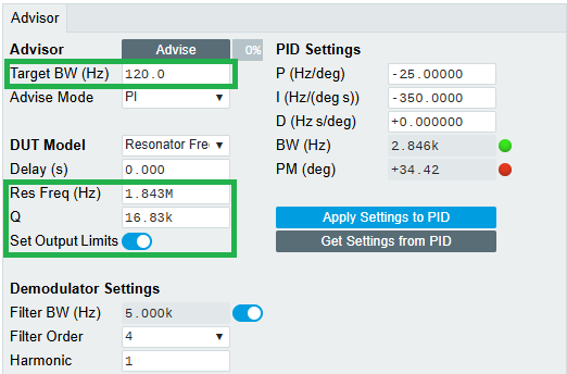
The PID Advisor finds suitable feedback gains by simulating the closed loop with a model of the device under test. Configure it as follows, as shown in Figure 17:

Set Target BW (Hz) to 120 Hz. The target bandwidth should be at least as large as the expected bandwidth of the frequency variations to be tracked. The resonance of this crystal is practically stable, so 120 Hz is sufficient.
Set Advise Mode to PI. A derivative term is not needed here.
Set DUT Model to Resonator frequency. The panel defaults to Internal PLL, which is the model for following an externally supplied oscillating signal rather than a passive resonator. Selecting the resonator model replaces the parameter fields with Res Freq and Q.
Enter the fitted values: Res Freq 1.8428 MHz and Q 16.83 k. Leave Delay at 0 s. It describes signal delay outside the instrument, about 5 ns per meter of coaxial cable, which is negligible at this target bandwidth.
Enable the toggle next to Filter BW (Hz) under Demodulator Settings. The Advisor then sets the demodulator bandwidth itself, to roughly five times the target bandwidth, so that demodulation speed does not limit the loop.
Click Advise.

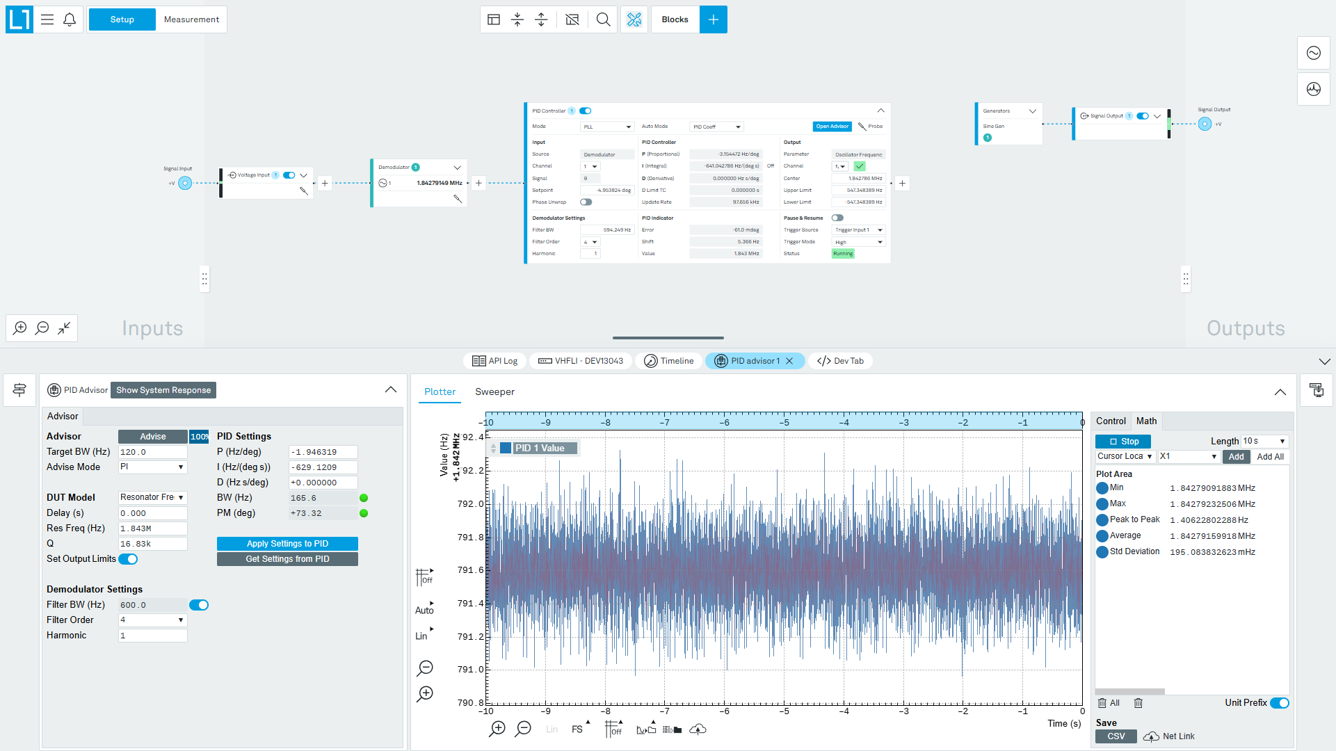
Figure 17: The Advisor configured with the target bandwidth, the Resonator frequency model with Res Freq and Q from the fit, and Set Output Limits enabled.

The Advisor runs a numerical optimization and reports the resulting gains together with the achieved bandwidth and phase margin, as shown in Figure 18. For this resonator it returns P = −1.946 Hz/deg and I = −629.121 Hz/(deg s), with an achieved bandwidth of 165.6 Hz and a phase margin of +73.32°.

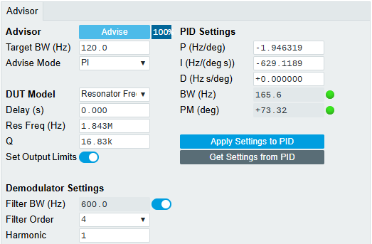
Figure 18: The PID Advisor after a successful run, showing the resulting feedback gains and the target-bandwidth and stability indicators, both green.

The two indicators next to the achieved bandwidth and phase margin in Figure 18 report whether the result is usable. The upper LED reports whether the target bandwidth can be achieved. If it is red, either lower the target bandwidth or reduce the delays in the loop. The lower LED reports whether the phase margin is sufficient for the loop to be stable. Both should be green before continuing.

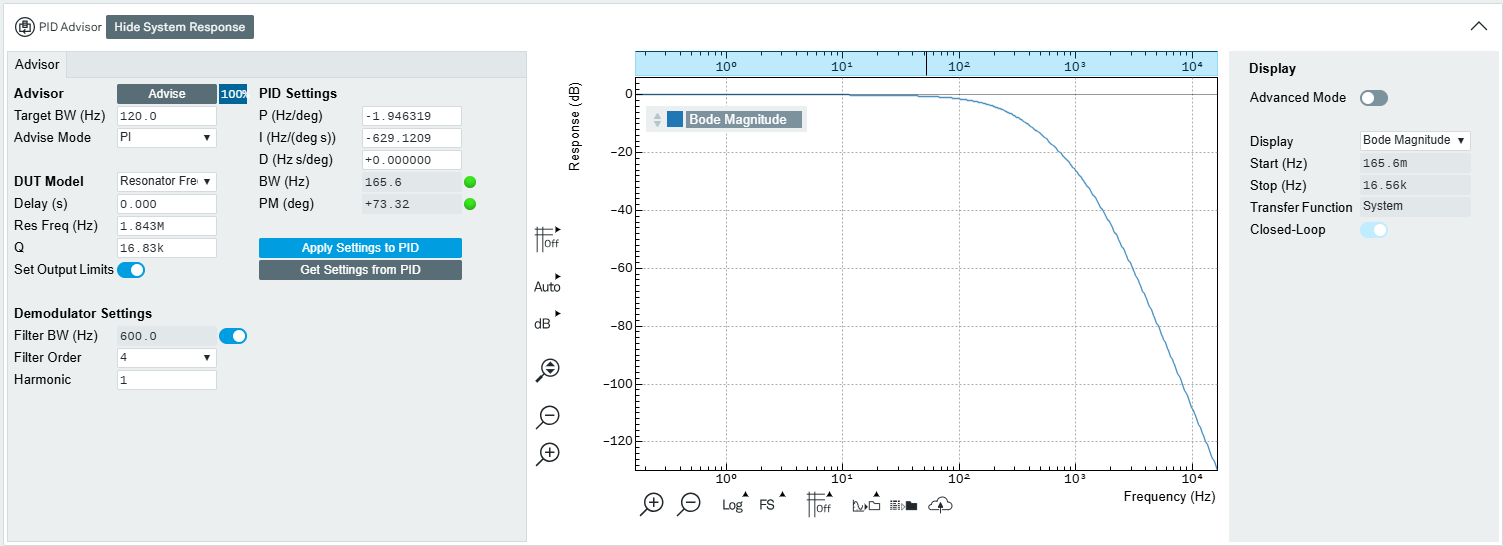
The simulated closed-loop response can be inspected with the Show System Response button, which plots the transfer function of the loop (Figure 19). The 3 dB point of the magnitude response corresponds to the achieved bandwidth reported by the Advisor.

Figure 19: Simulated closed-loop magnitude response of the PLL. The 3 dB point corresponds to the bandwidth reported by the Advisor.

When the result is satisfactory, click Apply Settings to PID to transfer the gains to the controller.

Track the Resonance¶

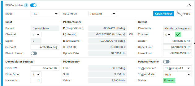
Switch the PID Controller on with the toggle in the block header. The PID Indicator section reports the state of the loop: Error is the difference between the measured phase and the setpoint, Shift is the frequency offset the controller has applied, and Value is the resulting oscillator frequency. A successful lock shows Error settling to a very small value, as in Figure 20.

Figure 20: The PID Controller enabled and locked. The small Error value indicates that the loop has settled.

Note

If the loop does not lock, check the signal input range. The auto-range button next to the Range field in the Voltage Input block picks the most sensitive setting that does not clip, which improves the signal-to-noise ratio available to the controller.

To watch the resonance frequency over time, use the Plotter in the PID advisor panel. In its signal selector, choose PID Value. This is the frequency the loop has settled on (Figure 21). The PID controller's data transfer is enabled automatically, so no further setup is needed. The neighboring signals are also useful: PID Shift is the same quantity expressed as an offset from the center frequency, and PID Error is the residual phase error.